hyperspy.external.astroML package¶

Submodules¶

hyperspy.external.astroML.bayesian_blocks module¶

Bayesian Block implementation¶

Dynamic programming algorithm for finding the optimal adaptive-width histogram.

Based on Scargle et al 2012 [1]_

References

[1]	http://adsabs.harvard.edu/abs/2012arXiv1207.5578S

class hyperspy.external.astroML.bayesian_blocks.Events(p0=0.05, gamma=None)¶

Bases: hyperspy.external.astroML.bayesian_blocks.FitnessFunc

Fitness for binned or unbinned events

Parameters:	p0 (float) – False alarm probability, used to compute the prior on N (see eq. 21 of Scargle 2012). Default prior is for p0 = 0. gamma (float or None) – If specified, then use this gamma to compute the general prior form, p ~ gamma^N. If gamma is specified, p0 is ignored.

fitness(N_k, T_k)¶

prior(N, Ntot)¶

class hyperspy.external.astroML.bayesian_blocks.FitnessFunc(p0=0.05, gamma=None)¶

Bases: object

Base class for fitness functions

Each fitness function class has the following: - fitness(...) : compute fitness function.

Arguments accepted by fitness must be among [T_k, N_k, a_k, b_k, c_k]

prior(N, Ntot) : compute prior on N given a total number of points Ntot

args¶

fitness(**kwargs)¶

gamma_prior(N, Ntot)¶: Basic prior, parametrized by gamma (eq. 3 in Scargle 2012)

p0_prior(N, Ntot)¶

prior(N, Ntot)¶

validate_input(t, x, sigma)¶: Check that input is valid

class hyperspy.external.astroML.bayesian_blocks.PointMeasures(p0=None, gamma=None)¶

Bases: hyperspy.external.astroML.bayesian_blocks.FitnessFunc

Fitness for point measures

Parameters:	gamma (float) – specifies the prior on the number of bins: p ~ gamma^N if gamma is not specified, then a prior based on simulations will be used (see sec 3.3 of Scargle 2012)

fitness(a_k, b_k)¶

prior(N, Ntot)¶

class hyperspy.external.astroML.bayesian_blocks.RegularEvents(dt, p0=0.05, gamma=None)¶

Bases: hyperspy.external.astroML.bayesian_blocks.FitnessFunc

Fitness for regular events

This is for data which has a fundamental “tick” length, so that all measured values are multiples of this tick length. In each tick, there are either zero or one counts.

Parameters:	dt (float) – tick rate for data gamma (float) – specifies the prior on the number of bins: p ~ gamma^N

fitness(T_k, N_k)¶

validate_input(t, x, sigma)¶

hyperspy.external.astroML.bayesian_blocks.bayesian_blocks(t, x=None, sigma=None, fitness='events', **kwargs)¶

Bayesian Blocks Implementation

This is a flexible implementation of the Bayesian Blocks algorithm described in Scargle 2012 [1]_

Parameters:	t (array_like) – data times (one dimensional, length N) x (array_like (optional)) – data values sigma (array_like or float (optional)) – data errors fitness (str or object) – the fitness function to use. If a string, the following options are supported: ‘events’ : binned or unbinned event data extra arguments are p0, which gives the false alarm probability to compute the prior, or gamma which gives the slope of the prior on the number of bins. ‘regular_events’ : non-overlapping events measured at multiples of a fundamental tick rate, dt, which must be specified as an additional argument. The prior can be specified through gamma, which gives the slope of the prior on the number of bins. ‘measures’ : fitness for a measured sequence with Gaussian errors The prior can be specified using gamma, which gives the slope of the prior on the number of bins. If gamma is not specified, then a simulation-derived prior will be used. Alternatively, the fitness can be a user-specified object of type derived from the FitnessFunc class.
Returns:	edges – array containing the (N+1) bin edges
Return type:	ndarray

Examples

Event data:

>>> t = np.random.normal(size=100)
>>> bins = bayesian_blocks(t, fitness='events', p0=0.01)

Event data with repeats:

>>> t = np.random.normal(size=100)
>>> t[80:] = t[:20]
>>> bins = bayesian_blocks(t, fitness='events', p0=0.01)

Regular event data:

>>> dt = 0.01
>>> t = dt * np.arange(1000)
>>> x = np.zeros(len(t))
>>> x[np.random.randint(0, len(t), len(t) / 10)] = 1
>>> bins = bayesian_blocks(t, fitness='regular_events', dt=dt, gamma=0.9)

Measured point data with errors:

>>> t = 100 * np.random.random(100)
>>> x = np.exp(-0.5 * (t - 50) ** 2)
>>> sigma = 0.1
>>> x_obs = np.random.normal(x, sigma)
>>> bins = bayesian_blocks(t, fitness='measures')

References

[1]	Scargle, J et al. (2012) http://adsabs.harvard.edu/abs/2012arXiv1207.5578S

See also

astroML.plotting.hist(): histogram plotting function which can make use of bayesian blocks.

hyperspy.external.astroML.histtools module¶

Tools for working with distributions

class hyperspy.external.astroML.histtools.KnuthF(data)¶

Bases: object

Class which implements the function minimized by knuth_bin_width

Parameters:	data (array-like, one dimension) – data to be histogrammed

Notes

the function F is given by

$F(M|x,I) = n\log(M) + \log\Gamma(\frac{M}{2}) - M\log\Gamma(\frac{1}{2}) - \log\Gamma(\frac{2n+M}{2}) + \sum_{k=1}^M \log\Gamma(n_k + \frac{1}{2})$

where $\Gamma$ is the Gamma function, $n$ is the number of data points, $n_k$ is the number of measurements in bin $k$ .

See also

knuth_bin_width, astroML.plotting.hist

bins(M)¶: Return the bin edges given a width dx

eval(M)¶

Evaluate the Knuth function

Parameters:	dx (float) – Width of bins
Returns:	F – evaluation of the negative Knuth likelihood function: smaller values indicate a better fit.
Return type:	float

hyperspy.external.astroML.histtools.freedman_bin_width(data, return_bins=False)¶

Return the optimal histogram bin width using the Freedman-Diaconis rule

Parameters:

data (array-like, ndim=1) – observed (one-dimensional) data
return_bins (bool (optional)) – if True, then return the bin edges

Returns:

width (float) – optimal bin width using Scott’s rule
bins (ndarray) – bin edges: returned if return_bins is True

Notes

The optimal bin width is

$\Delta_b = \frac{2(q_{75} - q_{25})}{n^{1/3}}$

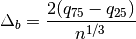
where $q_{N}$ is the $N$ percent quartile of the data, and $n$ is the number of data points.

See also

knuth_bin_width(), scotts_bin_width(), astroML.plotting.hist()

hyperspy.external.astroML.histtools.histogram(a, bins=10, range=None, **kwargs)¶

Enhanced histogram

This is a histogram function that enables the use of more sophisticated algorithms for determining bins. Aside from the bins argument allowing a string specified how bins are computed, the parameters are the same as numpy.histogram().

Parameters:

a (array_like) – array of data to be histogrammed
bins (int or list or str (optional)) – If bins is a string, then it must be one of: ‘blocks’ : use bayesian blocks for dynamic bin widths ‘knuth’ : use Knuth’s rule to determine bins ‘scotts’ : use Scott’s rule to determine bins ‘freedman’ : use the Freedman-diaconis rule to determine bins
range (tuple or None (optional)) – the minimum and maximum range for the histogram. If not specified, it will be (x.min(), x.max())
keyword arguments are described in numpy.hist(). (other) –

Returns:

hist (array) – The values of the histogram. See normed and weights for a description of the possible semantics.
bin_edges (array of dtype float) – Return the bin edges (length(hist)+1).

See also

numpy.histogram(), astroML.plotting.hist()

hyperspy.external.astroML.histtools.knuth_bin_width(data, return_bins=False)¶

Return the optimal histogram bin width using Knuth’s rule [1]_

Parameters:

data (array-like, ndim=1) – observed (one-dimensional) data
return_bins (bool (optional)) – if True, then return the bin edges

Returns:

dx (float) – optimal bin width. Bins are measured starting at the first data point.
bins (ndarray) – bin edges: returned if return_bins is True

Notes

The optimal number of bins is the value M which maximizes the function

$F(M|x,I) = n\log(M) + \log\Gamma(\frac{M}{2}) - M\log\Gamma(\frac{1}{2}) - \log\Gamma(\frac{2n+M}{2}) + \sum_{k=1}^M \log\Gamma(n_k + \frac{1}{2})$

where $\Gamma$ is the Gamma function, $n$ is the number of data points, $n_k$ is the number of measurements in bin $k$ .

References

[1]	Knuth, K.H. “Optimal Data-Based Binning for Histograms”. arXiv:0605197, 2006

hyperspy.external.astroML.histtools.scotts_bin_width(data, return_bins=False)¶

Return the optimal histogram bin width using Scott’s rule:

Parameters:

data (array-like, ndim=1) – observed (one-dimensional) data
return_bins (bool (optional)) – if True, then return the bin edges

Returns:

width (float) – optimal bin width using Scott’s rule
bins (ndarray) – bin edges: returned if return_bins is True

Notes

The optimal bin width is

$\Delta_b = \frac{3.5\sigma}{n^{1/3}}$

where $\sigma$ is the standard deviation of the data, and $n$ is the number of data points.

See also

knuth_bin_width(), freedman_bin_width(), astroML.plotting.hist()

hyperspy.external.astroML package¶

Submodules¶

hyperspy.external.astroML.bayesian_blocks module¶

Bayesian Block implementation¶

hyperspy.external.astroML.histtools module¶

Module contents¶