Machine learning
Introduction
HyperSpy provides easy access to several “machine learning” algorithms which can be useful when analysing multidimensional data. In particular, decomposition algorithms such as principal component analysis (PCA) or blind source separation (BSS) algorithms such as independent component analysis (ICA) are available through the methods described in this section.
The behaviour of some machine learning operations can be customised customised in the Machine Learning section Preferences.
Note
Currently the BSS algorithms operate on the result of a previous decomposition analysis. Therefore, it is necessary to perform a decomposition before attempting to perform a BSS.
Nomenclature
HyperSpy performs the decomposition of a dataset into two new datasets: one with the dimension of the signal space which we will call factors and the other with the dimension of the navigation space which we will call loadings. The same nomenclature applies to the result of BSS.
Decomposition
There are several methods to decompose a matrix or tensor into several factors.
The decomposition is most commonly applied as a means of noise reduction and
dimensionality reduction. One of the most popular decomposition methods is
principal component analysis (PCA). To perform PCA on your data set, run the
decomposition() method:
>>> s.decomposition()
Note that the s variable must contain a BaseSignal class or
any of its subclasses which most likely has been previously loaded with the
load() function, e.g. s = load('my_file.hdf5'). Also, the signal must be
multidimensional, i.e. s.axes_manager.navigation_size must be greater than
one.
Several algorithms exist for performing this analysis. The default algorithm in
HyperSpy is SVD, which performs PCA using an approach called
“singular value decomposition”. This method has many options. For more details
read method documentation.
Poissonian noise
Most decomposition algorithms assume that the noise of the data follows a Gaussian distribution. In the case that the data that you are analysing follow a Poissonian distribution instead, HyperSpy can “normalize” the data by performing a scaling operation which can greatly enhance the result.
To perform Poissonian noise normalisation:
The long way:
>>> s.decomposition(normalize_poissonian_noise=True)

Because it is the first argument we cold have simply written:
>>> s.decomposition(True)
For more details about the scaling procedure you can read the following research article
Principal component analysis
Scree plot
PCA essentially sorts the components in the data in order of decreasing variance. It is often useful to estimate the dimensionality of the data by plotting the explained variance against the component index in a logarithmic y-scale. This plot is sometimes called scree-plot and it should drop quickly, eventually becoming a slowly descending line. The point at which it becomes linear (often referred to as an elbow) is generally judged to be a good estimation of the dimensionality of the data (or equivalently, the number of components that should be retained - see below).
To obtain a scree plot, run the
plot_explained_variance_ratio() method e.g.:
>>> ax = s.plot_explained_variance_ratio()
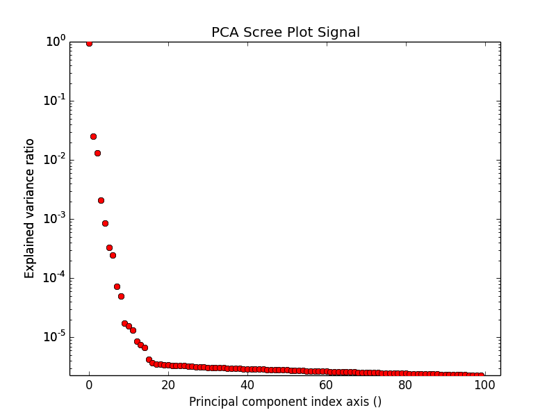
PCA scree plot.
Note that in the figure, the first component has index 0. This is because Python uses zero based indexing i.e. the initial element of a sequence is found using index 0.
New in version 0.7.
Sometimes it can be useful to get the explained variance ratio as a spectrum,
e.g. to store it separetely or to plot several scree plots obtained using
different data pre-treatment in the same figure using
plot_spectra(). For that you can use
get_explained_variance_ratio()
Data denoising (dimensionality reductions)
One of the most popular uses of PCA is data denoising. The denoising property is achieved by using a limited set of components to make a model of the original, omitting the later components that ideally contain only noise. This is know as dimensionality reduction.
To perform this operation with HyperSpy, run the
get_decomposition_model() method, usually after
estimating the dimension of your data e.g. by using the Scree plot. For
example:
>>> sc = s.get_decomposition_model(components)
Note
The components argument can be one of several things (None, int, or list of ints):
- if None, all the components are used to construct the model.
- if int, only the given number of components (starting from index 0) are used to construct the model.
- if list of ints, only the components in the given list are used to construct the model.
Hint
Unlike most of the analysis functions, this function returns a new
object, which in the example above we have called ‘sc’. (The name of
the variable is totally arbitrary and you can choose it at your will).
You can perform operations on this new object later. It is a copy of the
original s object, except that the data has been replaced by
the model constructed using the chosen components.
Sometimes it is useful to examine the residuals between your original data and the decomposition model. You can easily compute and display the residuals in one single line of code:
>>> (s - sc).plot()
Blind Source Separation
In some cases (it largely depends on the particular application) it is possible to obtain more physically meaningful components from the result of a data decomposition by a process called Blind Source Separation (BSS). For more information about the blind source separation you can read the following introductory article or this other article from the authors of HyperSpy for an application to EELS analysis.
To perform BSS on the result of a decomposition, run the
blind_source_separation() method, e.g.:
s.blind_source_separation(number_of_components)
Note
You must have performed a Decomposition before you attempt to perform BSS.
Note
You must pass an integer number of components to ICA. The best way to estimate this number in the case of a PCA decomposition is by inspecting the Scree plot.
Visualising results
Plot methods exist for the results of decomposition and blind source separation. All the methods begin with “plot”:
plot_decomposition_results().plot_decomposition_factors().plot_decomposition_loadings().plot_bss_results().plot_bss_factors().plot_bss_loadings().
1 and 4 (new in version 0.7) provide a more compact way of displaying the
results. All the other methods display each component in its own window. For 2
and 3 it is wise to provide the number of factors or loadings you wish to
visualise, since the default is plot all. For BSS the default is the number you
included when running the blind_source_separation()
method.
Obtaining the results as Signal instances
New in version 0.7.
The decomposition and BSS results are internally stored in the
BaseSignal class where all the methods discussed in this
chapter can find them. However, they are stored as numpy array. Frequently it
is useful to obtain the decomposition/BSS factors and loadings as HyperSpy
signals and HyperSpy provides the following four methods for that pourpose:
Saving and loading results
There are several methods for storing the result of a machine learning analysis.
Saving in the main file
When you save the object on which you’ve performed machine learning analysis in the HDF5 format (the default in HyperSpy) (see Saving data to files) the result of the analysis is automatically saved in the file and it is loaded with the rest of the data when you load the file.
This option is the simplest because everything is stored in the same file and it does not require any extra command to recover the result of machine learning analysis when loading a file. However, currently it only supports storing one decomposition and one BSS result, which may not be enough for your purposes.
Saving to an external files
Alternatively, to save the results of the current machine learning analysis to
a file you can use the save() method,
e.g.:
Save the result of the analysis
>>> s.learning_results.save('my_results')

Load back the results
>>> s.learning_results.load('my_results.npz')
Exporting
It is possible to export the results of machine learning to any format supported by HyperSpy using:
These methods accept many arguments which can be used to customise the way the data is exported, so please consult the method documentation. The options include the choice of file format, the prefixes for loadings and factors, saving figures instead of data and more.
Please note that the exported data cannot easily be loaded into HyperSpy’s machine learning structure.