hyperspy.signal module¶

class hyperspy.signal.BaseSetMetadataItems(signal)¶

Bases: traits.has_traits.HasTraits

store(*args, **kwargs)¶

class hyperspy.signal.BaseSignal(data, **kwds)¶

Bases: hyperspy.misc.slicing.FancySlicing, hyperspy.learn.mva.MVA, hyperspy.signal.MVATools

Create a Signal from a numpy array.

Parameters

data (numpy.ndarray) – The signal data. It can be an array of any dimensions.
axes (dict, optional) – Dictionary to define the axes (see the documentation of the AxesManager class for more details).
attributes (dict, optional) – A dictionary whose items are stored as attributes.
metadata (dict, optional) – A dictionary containing a set of parameters that will to stores in the metadata attribute. Some parameters might be mandatory in some cases.
original_metadata (dict, optional) – A dictionary containing a set of parameters that will to stores in the original_metadata attribute. It typically contains all the parameters that has been imported from the original data file.

property T¶: The transpose of the signal, with signal and navigation spaces swapped. Enables calling transpose() with the default parameters as a property of a Signal.

add_gaussian_noise(std)¶

Add Gaussian noise to the data.

The operation is performed in-place (i.e. the data of the signal is modified). This method requires a float data type, otherwise numpy raises a TypeError.

Parameters: std (float) – The standard deviation of the Gaussian noise.

Note

This method uses numpy.random.normal() (or dask.array.random.normal() for lazy signals) to generate the Gaussian noise. In order to seed it, you must use numpy.random.seed().

add_marker(marker, plot_on_signal=True, plot_marker=True, permanent=False, plot_signal=True, render_figure=True)¶

Add one or several markers to the signal or navigator plot and plot the signal, if not yet plotted (by default)

Parameters

marker (hyperspy.drawing.marker object or iterable) – The marker or iterable (list, tuple, …) of markers to add. See the Markers section in the User Guide if you want to add a large number of markers as an iterable, since this will be much faster. For signals with navigation dimensions, the markers can be made to change for different navigation indices. See the examples for info.
plot_on_signal (bool) – If True (default), add the marker to the signal. If False, add the marker to the navigator
plot_marker (bool) – If True (default), plot the marker.
permanent (bool) – If False (default), the marker will only appear in the current plot. If True, the marker will be added to the metadata.Markers list, and be plotted with plot(plot_markers=True). If the signal is saved as a HyperSpy HDF5 file, the markers will be stored in the HDF5 signal and be restored when the file is loaded.

Examples

>>> import scipy.misc
>>> im = hs.signals.Signal2D(scipy.misc.ascent())
>>> m = hs.markers.rectangle(x1=150, y1=100, x2=400,
>>>                                  y2=400, color='red')
>>> im.add_marker(m)

Adding to a 1D signal, where the point will change when the navigation index is changed:

>>> s = hs.signals.Signal1D(np.random.random((3, 100)))
>>> marker = hs.markers.point((19, 10, 60), (0.2, 0.5, 0.9))
>>> s.add_marker(marker, permanent=True, plot_marker=True)

Add permanent marker:

>>> s = hs.signals.Signal2D(np.random.random((100, 100)))
>>> marker = hs.markers.point(50, 60, color='red')
>>> s.add_marker(marker, permanent=True, plot_marker=True)

Add permanent marker to signal with 2 navigation dimensions. The signal has navigation dimensions (3, 2), as the dimensions gets flipped compared to the output from numpy.random.random(). To add a vertical line marker which changes for different navigation indices, the list used to make the marker must be a nested list: 2 lists with 3 elements each (2 x 3):

>>> s = hs.signals.Signal1D(np.random.random((2, 3, 10)))
>>> marker = hs.markers.vertical_line([[1, 3, 5], [2, 4, 6]])
>>> s.add_marker(marker, permanent=True)

Add permanent marker which changes with navigation position, and do not add it to a current plot:

>>> s = hs.signals.Signal2D(np.random.randint(10, size=(3, 100, 100)))
>>> marker = hs.markers.point((10, 30, 50), (30, 50, 60), color='red')
>>> s.add_marker(marker, permanent=True, plot_marker=False)
>>> s.plot(plot_markers=True) #doctest: +SKIP

Removing a permanent marker:

>>> s = hs.signals.Signal2D(np.random.randint(10, size=(100, 100)))
>>> marker = hs.markers.point(10, 60, color='red')
>>> marker.name = "point_marker"
>>> s.add_marker(marker, permanent=True)
>>> del s.metadata.Markers.point_marker

Adding many markers as a list:

>>> from numpy.random import random
>>> s = hs.signals.Signal2D(np.random.randint(10, size=(100, 100)))
>>> marker_list = []
>>> for i in range(100):
>>>     marker = hs.markers.point(random()*100, random()*100, color='red')
>>>     marker_list.append(marker)
>>> s.add_marker(marker_list, permanent=True)

add_poissonian_noise(keep_dtype=True)¶

Add Poissonian noise to the data

This method works in-place. The resulting data type is int64. If this is different from the original data type a warning is added to the log.

Parameters: keep_dtype (bool) – If True, keep the original data type of the signal data. For example, if the data type was initially 'float64', the result of the operation (usually 'int64') will be converted to 'float64'. The default is True for convenience.

Note

This method uses numpy.random.poisson() (or dask.array.random.poisson() for lazy signals) to generate the Gaussian noise. In order to seed it, you must use numpy.random.seed().

apply_apodization(window='hann', hann_order=None, tukey_alpha=0.5, inplace=False)¶

Apply an apodization window to a Signal.

Parameters

window (str, optional) – Select between {'hann' (default), 'hamming', or 'tukey'}
hann_order (None or int, optional) – Only used if window='hann' If integer n is provided, a Hann window of n-th order will be used. If None, a first order Hann window is used. Higher orders result in more homogeneous intensity distribution.
tukey_alpha (float, optional) –
Only used if window='tukey' (default is 0.5). From the documentation of scipy.signal.windows.tukey():
- Shape parameter of the Tukey window, representing the fraction of the window inside the cosine tapered region. If zero, the Tukey window is equivalent to a rectangular window. If one, the Tukey window is equivalent to a Hann window.
inplace (bool, optional) – If True, the apodization is applied in place, i.e. the signal data will be substituted by the apodized one (default is False).

Returns

out – If inplace=False, returns the apodized signal of the same type as the provided Signal.

Return type

BaseSignal (or subclasses), optional

Examples

>>> import hyperspy.api as hs
>>> holo = hs.datasets.example_signals.object_hologram()
>>> holo.apply_apodization('tukey', tukey_alpha=0.1).plot()

as_lazy(copy_variance=True)¶

Create a copy of the given Signal as a LazySignal.

Parameters: copy_variance (bool) – Whether or not to copy the variance from the original Signal to the new lazy version
Returns: res – The same signal, converted to be lazy
Return type: LazySignal

as_signal1D(spectral_axis, out=None, optimize=True)¶

Return the Signal as a spectrum.

The chosen spectral axis is moved to the last index in the array and the data is made contiguous for efficient iteration over spectra. By default, the method ensures the data is stored optimally, hence often making a copy of the data. See transpose() for a more general method with more options.

Parameters

spectral_axis (int, str, or DataAxis) – The axis can be passed directly, or specified using the index of the axis in the Signal’s axes_manager or the axis name.
out (BaseSignal (or subclasses) or None) – If None, a new Signal is created with the result of the operation and returned (default). If a Signal is passed, it is used to receive the output of the operation, and nothing is returned.
optimize (bool) – If True, the location of the data in memory is optimised for the fastest iteration over the navigation axes. This operation can cause a peak of memory usage and requires considerable processing times for large datasets and/or low specification hardware. See the Transposing (changing signal spaces) section of the HyperSpy user guide for more information. When operating on lazy signals, if True, the chunks are optimised for the new axes configuration.

Examples

>>> img = hs.signals.Signal2D(np.ones((3,4,5,6)))
>>> img
<Signal2D, title: , dimensions: (4, 3, 6, 5)>
>>> img.as_signal1D(-1+1j)
<Signal1D, title: , dimensions: (6, 5, 4, 3)>
>>> img.as_signal1D(0)
<Signal1D, title: , dimensions: (6, 5, 3, 4)>

as_signal2D(image_axes, out=None, optimize=True)¶

Convert a signal to image ( Signal2D).

The chosen image axes are moved to the last indices in the array and the data is made contiguous for efficient iteration over images.

Parameters

image_axes (tuple (of int, str or DataAxis)) – Select the image axes. Note that the order of the axes matters and it is given in the “natural” i.e. X, Y, Z… order.
out (BaseSignal (or subclasses) or None) – If None, a new Signal is created with the result of the operation and returned (default). If a Signal is passed, it is used to receive the output of the operation, and nothing is returned.
optimize (bool) – If True, the location of the data in memory is optimised for the fastest iteration over the navigation axes. This operation can cause a peak of memory usage and requires considerable processing times for large datasets and/or low specification hardware. See the Transposing (changing signal spaces) section of the HyperSpy user guide for more information. When operating on lazy signals, if True, the chunks are optimised for the new axes configuration.

Raises

DataDimensionError – when data.ndim < 2

Examples

>>> s = hs.signals.Signal1D(np.ones((2,3,4,5)))
>>> s
<Signal1D, title: , dimensions: (4, 3, 2, 5)>
>>> s.as_signal2D((0,1))
<Signal2D, title: , dimensions: (5, 2, 4, 3)>

>>> s.to_signal2D((1,2))
<Signal2D, title: , dimensions: (4, 5, 3, 2)>

change_dtype(dtype, rechunk=True)¶

Change the data type of a Signal.

Parameters

dtype (str or numpy.dtype) – Typecode string or data-type to which the Signal’s data array is cast. In addition to all the standard numpy Data type objects (dtype), HyperSpy supports four extra dtypes for RGB images: 'rgb8', 'rgba8', 'rgb16', and 'rgba16'. Changing from and to any rgb(a) dtype is more constrained than most other dtype conversions. To change to an rgb(a) dtype, the signal_dimension must be 1, and its size should be 3 (for rgb) or 4 (for rgba) dtypes. The original dtype should be uint8 or uint16 if converting to rgb(a)8 or rgb(a))16, and the navigation_dimension should be at least 2. After conversion, the signal_dimension becomes 2. The dtype of images with original dtype rgb(a)8 or rgb(a)16 can only be changed to uint8 or uint16, and the signal_dimension becomes 1.
rechunk (bool) – Only has effect when operating on lazy signal. If True (default), the data may be automatically rechunked before performing this operation.

Examples

>>> s = hs.signals.Signal1D([1,2,3,4,5])
>>> s.data
array([1, 2, 3, 4, 5])
>>> s.change_dtype('float')
>>> s.data
array([ 1.,  2.,  3.,  4.,  5.])

copy()¶: Return a “shallow copy” of this Signal using the standard library’s copy() function. Note: this will return a copy of the signal, but it will not duplicate the underlying data in memory, and both Signals will reference the same data.

crop(axis, start=None, end=None, convert_units=False)¶

Crops the data in a given axis. The range is given in pixels.

Parameters

axis (int or str) – Specify the data axis in which to perform the cropping operation. The axis can be specified using the index of the axis in axes_manager or the axis name.
start (int, float, or None) – The beginning of the cropping interval. If type is int, the value is taken as the axis index. If type is float the index is calculated using the axis calibration. If start/end is None the method crops from/to the low/high end of the axis.
end (int, float, or None) – The end of the cropping interval. If type is int, the value is taken as the axis index. If type is float the index is calculated using the axis calibration. If start/end is None the method crops from/to the low/high end of the axis.
convert_units (bool) – Default is False. If True, convert the units using the convert_units() method of the AxesManager. If False, does nothing.

property data¶: The underlying data structure as a numpy.ndarray (or dask.array.Array, if the Signal is lazy).

deepcopy()¶: Return a “deep copy” of this Signal using the standard library’s deepcopy() function. Note: this means the underlying data structure will be duplicated in memory.

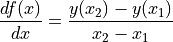
derivative(axis, order=1, out=None, rechunk=True)¶

Calculate the numerical derivative along the given axis, with respect to the calibrated units of that axis.

For a function $y = f(x)$ and two consecutive values $x_1$ and $x_2$ :

$\frac{df(x)}{dx} = \frac{y(x_2)-y(x_1)}{x_2-x_1}$

Parameters

axis (int, str, or DataAxis) – The axis can be passed directly, or specified using the index of the axis in the Signal’s axes_manager or the axis name.
order (int) – The order of the derivative.
out (BaseSignal (or subclasses) or None) – If None, a new Signal is created with the result of the operation and returned (default). If a Signal is passed, it is used to receive the output of the operation, and nothing is returned.
rechunk (bool) – Only has effect when operating on lazy signal. If True (default), the data may be automatically rechunked before performing this operation.

Returns

der – Note that the size of the data on the given axis decreases by the given order. i.e. if axis is "x" and order is 2, if the x dimension is N, then der’s x dimension is N - 2.

Return type

BaseSignal

diff(axis, order=1, out=None, rechunk=True)¶

Returns a signal with the n-th order discrete difference along given axis. i.e. it calculates the difference between consecutive values in the given axis: out[n] = a[n+1] - a[n]. See numpy.diff() for more details.

Parameters

axis (int, str, or DataAxis) – The axis can be passed directly, or specified using the index of the axis in the Signal’s axes_manager or the axis name.
order (int) – The order of the discrete difference.
out (BaseSignal (or subclasses) or None) – If None, a new Signal is created with the result of the operation and returned (default). If a Signal is passed, it is used to receive the output of the operation, and nothing is returned.
rechunk (bool) – Only has effect when operating on lazy signal. If True (default), the data may be automatically rechunked before performing this operation.

Returns

s – Note that the size of the data on the given axis decreases by the given order. i.e. if axis is "x" and order is 2, the x dimension is N, der’s x dimension is N - 2.

Return type

BaseSignal (or subclasses) or None

Examples

>>> import numpy as np
>>> s = BaseSignal(np.random.random((64,64,1024)))
>>> s.data.shape
(64,64,1024)
>>> s.diff(-1).data.shape
(64,64,1023)

estimate_poissonian_noise_variance(expected_value=None, gain_factor=None, gain_offset=None, correlation_factor=None)¶

Estimate the Poissonian noise variance of the signal.

The variance is stored in the metadata.Signal.Noise_properties.variance attribute.

The Poissonian noise variance is equal to the expected value. With the default arguments, this method simply sets the variance attribute to the given expected_value. However, more generally (although then the noise is not strictly Poissonian), the variance may be proportional to the expected value. Moreover, when the noise is a mixture of white (Gaussian) and Poissonian noise, the variance is described by the following linear model:

$\mathrm{Var}[X] = (a * \mathrm{E}[X] + b) * c$

Where a is the gain_factor, b is the gain_offset (the Gaussian noise variance) and c the correlation_factor. The correlation factor accounts for correlation of adjacent signal elements that can be modeled as a convolution with a Gaussian point spread function.

Parameters

expected_value (None or BaseSignal (or subclasses)) – If None, the signal data is taken as the expected value. Note that this may be inaccurate where the value of data is small.
gain_factor (None or float) – a in the above equation. Must be positive. If None, take the value from metadata.Signal.Noise_properties.Variance_linear_model if defined. Otherwise, suppose pure Poissonian noise (i.e. gain_factor=1). If not None, the value is stored in metadata.Signal.Noise_properties.Variance_linear_model.
gain_offset (None or float) – b in the above equation. Must be positive. If None, take the value from metadata.Signal.Noise_properties.Variance_linear_model if defined. Otherwise, suppose pure Poissonian noise (i.e. gain_offset=0). If not None, the value is stored in metadata.Signal.Noise_properties.Variance_linear_model.
correlation_factor (None or float) – c in the above equation. Must be positive. If None, take the value from metadata.Signal.Noise_properties.Variance_linear_model if defined. Otherwise, suppose pure Poissonian noise (i.e. correlation_factor=1). If not None, the value is stored in metadata.Signal.Noise_properties.Variance_linear_model.

fft(shift=False, apodization=False, **kwargs)¶

Compute the discrete Fourier Transform.

This function computes the discrete Fourier Transform over the signal axes by means of the Fast Fourier Transform (FFT) as implemented in numpy.

Parameters

shift (bool, optional) – If True, the origin of FFT will be shifted to the centre (default is False).
apodization (bool or str) –
Apply an apodization window before calculating the FFT in order to suppress streaks. Valid string values are {'hann' or 'hamming' or 'tukey'} If True or 'hann', applies a Hann window. If 'hamming' or 'tukey', applies Hamming or Tukey windows, respectively (default is False).
**kwargs (dict) – other keyword arguments are described in numpy.fft.fftn()

Returns

s – A Signal containing the result of the FFT algorithm

Return type

ComplexSignal

Examples

>>> im = hs.signals.Signal2D(scipy.misc.ascent())
>>> im.fft()
<ComplexSignal2D, title: FFT of , dimensions: (|512, 512)>

>>> # Use following to plot power spectrum of `im`:
>>> im.fft(shift=True, apodization=True).plot(power_spectrum=True)

Note

For further information see the documentation of numpy.fft.fftn()

fold()¶: If the signal was previously unfolded, fold it back

get_current_signal(auto_title=True, auto_filename=True)¶

Returns the data at the current coordinates as a BaseSignal subclass.

The signal subclass is the same as that of the current object. All the axes navigation attributes are set to False.

Parameters

auto_title (bool) – If True, the current indices (in parentheses) are appended to the title, separated by a space.
auto_filename (bool) – If True and tmp_parameters.filename is defined (which is always the case when the Signal has been read from a file), the filename stored in the metadata is modified by appending an underscore and the current indices in parentheses.

Returns

cs – The data at the current coordinates as a Signal

Return type

BaseSignal (or subclass)

Examples

>>> im = hs.signals.Signal2D(np.zeros((2,3, 32,32)))
>>> im
<Signal2D, title: , dimensions: (3, 2, 32, 32)>
>>> im.axes_manager.indices = 2,1
>>> im.get_current_signal()
<Signal2D, title:  (2, 1), dimensions: (32, 32)>

get_dimensions_from_data()¶: Get the dimension parameters from the Signal’s underlying data. Useful when the data structure was externally modified, or when the spectrum image was not loaded from a file

get_histogram(bins='freedman', range_bins=None, out=None, **kwargs)¶

Return a histogram of the signal data.

More sophisticated algorithms for determining bins can be used. Aside from the bins argument allowing a string specified how bins are computed, the parameters are the same as numpy.histogram().

Parameters

bins (int, list, or str, optional) –
If bins is a string, then it must be one of:
- 'knuth' : use Knuth’s rule to determine bins
- 'scotts' : use Scott’s rule to determine bins
- 'freedman' : use the Freedman-diaconis rule to determine bins
- 'blocks' : use bayesian blocks for dynamic bin widths
range_bins (tuple or None, optional) – the minimum and maximum range for the histogram. If range_bins is None, (x.min(), x.max()) will be used.
out (BaseSignal (or subclasses) or None) – If None, a new Signal is created with the result of the operation and returned (default). If a Signal is passed, it is used to receive the output of the operation, and nothing is returned.
rechunk (bool) – Only has effect when operating on lazy signal. If True (default), the data may be automatically rechunked before performing this operation.
**kwargs – other keyword arguments (weight and density) are described in numpy.histogram().

Returns

hist_spec – A 1D spectrum instance containing the histogram.

Return type

Signal1D

Notes

The lazy version of the algorithm does not support the 'knuth' and 'blocks' bins arguments.
The estimators for bins are taken from the AstroML project. Read the documentation of astroML.density_estimation.histogram() for more info.

Examples

>>> s = hs.signals.Signal1D(np.random.normal(size=(10, 100)))
>>> # Plot the data histogram
>>> s.get_histogram().plot()
>>> # Plot the histogram of the signal at the current coordinates
>>> s.get_current_signal().get_histogram().plot()

ifft(shift=None, **kwargs)¶

Compute the inverse discrete Fourier Transform.

This function computes the real part of the inverse of the discrete Fourier Transform over the signal axes by means of the Fast Fourier Transform (FFT) as implemented in numpy.

Parameters

shift (bool or None, optional) – If None, the shift option will be set to the original status of the FFT using the value in metadata. If no FFT entry is present in metadata, the parameter will be set to False. If True, the origin of the FFT will be shifted to the centre. If False, the origin will be kept at (0, 0) (default is None).
**kwargs (dict) – other keyword arguments are described in numpy.fft.ifftn()

Returns

s – A Signal containing the result of the inverse FFT algorithm

Return type

BaseSignal (or subclasses)

Examples

>>> import scipy
>>> im = hs.signals.Signal2D(scipy.misc.ascent())
>>> imfft = im.fft()
>>> imfft.ifft()
<Signal2D, title: real(iFFT of FFT of ), dimensions: (|512, 512)>

Note

For further information see the documentation of numpy.fft.ifftn()

indexmax(axis, out=None, rechunk=True)¶

Returns a signal with the index of the maximum along an axis.

Parameters

axis (int, str, or DataAxis) – The axis can be passed directly, or specified using the index of the axis in the Signal’s axes_manager or the axis name.
out (BaseSignal (or subclasses) or None) – If None, a new Signal is created with the result of the operation and returned (default). If a Signal is passed, it is used to receive the output of the operation, and nothing is returned.
rechunk (bool) – Only has effect when operating on lazy signal. If True (default), the data may be automatically rechunked before performing this operation.

Returns

s – A new Signal containing the indices of the maximum along the specified axis. Note: the data dtype is always int.

Return type

BaseSignal (or subclasses)

Examples

>>> import numpy as np
>>> s = BaseSignal(np.random.random((64,64,1024)))
>>> s.data.shape
(64,64,1024)
>>> s.indexmax(-1).data.shape
(64,64)

indexmin(axis, out=None, rechunk=True)¶

Returns a signal with the index of the minimum along an axis.

Parameters

axis (int, str, or DataAxis) – The axis can be passed directly, or specified using the index of the axis in the Signal’s axes_manager or the axis name.
out (BaseSignal (or subclasses) or None) – If None, a new Signal is created with the result of the operation and returned (default). If a Signal is passed, it is used to receive the output of the operation, and nothing is returned.
rechunk (bool) – Only has effect when operating on lazy signal. If True (default), the data may be automatically rechunked before performing this operation.

Returns

s – A new Signal containing the indices of the minimum along the specified axis. Note: the data dtype is always int.

Return type

BaseSignal (or subclasses)

Examples

>>> import numpy as np
>>> s = BaseSignal(np.random.random((64,64,1024)))
>>> s.data.shape
(64,64,1024)
>>> s.indexmin(-1).data.shape
(64,64)

integrate1D(axis, out=None)¶

Integrate the signal over the given axis.

The integration is performed using Simpson’s rule if metadata.Signal.binned is False and simple summation over the given axis if True.

Parameters

axis (int, str, or DataAxis) – The axis can be passed directly, or specified using the index of the axis in the Signal’s axes_manager or the axis name.
out (BaseSignal (or subclasses) or None) – If None, a new Signal is created with the result of the operation and returned (default). If a Signal is passed, it is used to receive the output of the operation, and nothing is returned.

Returns

s – A new Signal containing the integral of the provided Signal along the specified axis.

Return type

BaseSignal (or subclasses)

Examples

>>> import numpy as np
>>> s = BaseSignal(np.random.random((64,64,1024)))
>>> s.data.shape
(64,64,1024)
>>> s.integrate1D(-1).data.shape
(64,64)

integrate_simpson(axis, out=None)¶

Calculate the integral of a Signal along an axis using Simpson’s rule.

Parameters

axis (int, str, or DataAxis) – The axis can be passed directly, or specified using the index of the axis in the Signal’s axes_manager or the axis name.
out (BaseSignal (or subclasses) or None) – If None, a new Signal is created with the result of the operation and returned (default). If a Signal is passed, it is used to receive the output of the operation, and nothing is returned.

Returns

s – A new Signal containing the integral of the provided Signal along the specified axis.

Return type

BaseSignal (or subclasses)

Examples

>>> import numpy as np
>>> s = BaseSignal(np.random.random((64,64,1024)))
>>> s.data.shape
(64,64,1024)
>>> s.integrate_simpson(-1).data.shape
(64,64)

property is_rgb¶: Whether or not this signal is an RGB dtype.

property is_rgba¶: Whether or not this signal is an RGB + alpha channel dtype.

property is_rgbx¶: Whether or not this signal is either an RGB or RGB + alpha channel dtype.

map(function, show_progressbar=None, parallel=None, inplace=True, ragged=None, **kwargs)¶

Apply a function to the signal data at all the navigation coordinates.

The function must operate on numpy arrays. It is applied to the data at each navigation coordinate pixel-py-pixel. Any extra keyword arguments are passed to the function. The keywords can take different values at different coordinates. If the function takes an axis or axes argument, the function is assumed to be vectorized and the signal axes are assigned to axis or axes. Otherwise, the signal is iterated over the navigation axes and a progress bar is displayed to monitor the progress.

In general, only navigation axes (order, calibration, and number) are guaranteed to be preserved.

Parameters

function (function) – Any function that can be applied to the signal.
show_progressbar (None or bool) – If True, display a progress bar. If None, the default from the preferences settings is used.
parallel (None or bool) – If True, perform computation in parallel using multiple cores. If None, the default from the preferences settings is used.
inplace (bool) – if True (default), the data is replaced by the result. Otherwise a new Signal with the results is returned.
ragged (None or bool) – Indicates if the results for each navigation pixel are of identical shape (and/or numpy arrays to begin with). If None, the appropriate choice is made while processing. Note: None is not allowed for Lazy signals!
**kwargs (dict) – All extra keyword arguments are passed to the provided function

Notes

If the function results do not have identical shapes, the result is an array of navigation shape, where each element corresponds to the result of the function (of arbitrary object type), called a “ragged array”. As such, most functions are not able to operate on the result and the data should be used directly.

This method is similar to Python’s map() that can also be utilized with a BaseSignal instance for similar purposes. However, this method has the advantage of being faster because it iterates the underlying numpy data array instead of the BaseSignal.

Examples

Apply a Gaussian filter to all the images in the dataset. The sigma parameter is constant:

>>> import scipy.ndimage
>>> im = hs.signals.Signal2D(np.random.random((10, 64, 64)))
>>> im.map(scipy.ndimage.gaussian_filter, sigma=2.5)

Apply a Gaussian filter to all the images in the dataset. The signal parameter is variable:

>>> im = hs.signals.Signal2D(np.random.random((10, 64, 64)))
>>> sigmas = hs.signals.BaseSignal(np.linspace(2,5,10)).T
>>> im.map(scipy.ndimage.gaussian_filter, sigma=sigmas)

max(axis=None, out=None, rechunk=True)¶

Returns a signal with the maximum of the signal along at least one axis.

Parameters

axis (int, str, DataAxis, tuple (of DataAxis) or None) – Either one on its own, or many axes in a tuple can be passed. In both cases the axes can be passed directly, or specified using the index in axes_manager or the name of the axis. Any duplicates are removed. If None, the operation is performed over all navigation axes (default).
out (BaseSignal (or subclasses) or None) – If None, a new Signal is created with the result of the operation and returned (default). If a Signal is passed, it is used to receive the output of the operation, and nothing is returned.
rechunk (bool) – Only has effect when operating on lazy signal. If True (default), the data may be automatically rechunked before performing this operation.

Returns

s – A new Signal containing the maximum of the provided Signal over the specified axes

Return type

BaseSignal (or subclasses)

Examples

>>> import numpy as np
>>> s = BaseSignal(np.random.random((64,64,1024)))
>>> s.data.shape
(64,64,1024)
>>> s.max(-1).data.shape
(64,64)

mean(axis=None, out=None, rechunk=True)¶

Returns a signal with the average of the signal along at least one axis.

Parameters

axis (int, str, DataAxis, tuple (of DataAxis) or None) – Either one on its own, or many axes in a tuple can be passed. In both cases the axes can be passed directly, or specified using the index in axes_manager or the name of the axis. Any duplicates are removed. If None, the operation is performed over all navigation axes (default).
out (BaseSignal (or subclasses) or None) – If None, a new Signal is created with the result of the operation and returned (default). If a Signal is passed, it is used to receive the output of the operation, and nothing is returned.
rechunk (bool) – Only has effect when operating on lazy signal. If True (default), the data may be automatically rechunked before performing this operation.

Returns

s – A new Signal containing the mean of the provided Signal over the specified axes

Return type

BaseSignal (or subclasses)

Examples

>>> import numpy as np
>>> s = BaseSignal(np.random.random((64,64,1024)))
>>> s.data.shape
(64,64,1024)
>>> s.mean(-1).data.shape
(64,64)

min(axis=None, out=None, rechunk=True)¶

Returns a signal with the minimum of the signal along at least one axis.

Parameters

axis (int, str, DataAxis, tuple (of DataAxis) or None) – Either one on its own, or many axes in a tuple can be passed. In both cases the axes can be passed directly, or specified using the index in axes_manager or the name of the axis. Any duplicates are removed. If None, the operation is performed over all navigation axes (default).
out (BaseSignal (or subclasses) or None) – If None, a new Signal is created with the result of the operation and returned (default). If a Signal is passed, it is used to receive the output of the operation, and nothing is returned.
rechunk (bool) – Only has effect when operating on lazy signal. If True (default), the data may be automatically rechunked before performing this operation.

Returns

s – A new Signal containing the minimum of the provided Signal over the specified axes

Return type

BaseSignal (or subclasses)

Examples

>>> import numpy as np
>>> s = BaseSignal(np.random.random((64,64,1024)))
>>> s.data.shape
(64,64,1024)
>>> s.min(-1).data.shape
(64,64)

nanmax(axis=None, out=None, rechunk=True)¶: Identical to max(), except ignores missing (NaN) values. See that method’s documentation for details.

nanmean(axis=None, out=None, rechunk=True)¶: Identical to mean(), except ignores missing (NaN) values. See that method’s documentation for details.

nanmin(axis=None, out=None, rechunk=True)¶: Identical to min(), except ignores missing (NaN) values. See that method’s documentation for details.

nanstd(axis=None, out=None, rechunk=True)¶: Identical to std(), except ignores missing (NaN) values. See that method’s documentation for details.

nansum(axis=None, out=None, rechunk=True)¶: Identical to sum(), except ignores missing (NaN) values. See that method’s documentation for details.

nanvar(axis=None, out=None, rechunk=True)¶: Identical to var(), except ignores missing (NaN) values. See that method’s documentation for details.

plot(navigator='auto', axes_manager=None, plot_markers=True, **kwargs)¶

Plot the signal at the current coordinates.

For multidimensional datasets an optional figure, the “navigator”, with a cursor to navigate that data is raised. In any case it is possible to navigate the data using the sliders. Currently only signals with signal_dimension equal to 0, 1 and 2 can be plotted.

Parameters

navigator (str, None, or BaseSignal (or subclass)) –

Allowed string values are 'auto', 'slider', and 'spectrum'.

If 'auto':

If navigation_dimension > 0, a navigator is provided to explore the data.

If navigation_dimension is 1 and the signal is an image the navigator is a sum spectrum obtained by integrating over the signal axes (the image).

If navigation_dimension is 1 and the signal is a spectrum the navigator is an image obtained by stacking all the spectra in the dataset horizontally.

If navigation_dimension is > 1, the navigator is a sum image obtained by integrating the data over the signal axes.

Additionally, if navigation_dimension > 2, a window with one slider per axis is raised to navigate the data.

For example, if the dataset consists of 3 navigation axes X, Y, Z and one signal axis, E, the default navigator will be an image obtained by integrating the data over E at the current Z index and a window with sliders for the X, Y, and Z axes will be raised. Notice that changing the Z-axis index changes the navigator in this case.

If 'slider':

If navigation dimension > 0 a window with one slider per axis is raised to navigate the data.

If 'spectrum':

If navigation_dimension > 0 the navigator is always a spectrum obtained by integrating the data over all other axes.

If None, no navigator will be provided.

Alternatively a BaseSignal (or subclass) instance can be provided. The signal_dimension must be 1 (for a spectrum navigator) or 2 (for a image navigator) and navigation_shape must be 0 (for a static navigator) or navigation_shape + signal_shape must be equal to the navigator_shape of the current object (for a dynamic navigator). If the signal dtype is RGB or RGBA this parameter has no effect and the value is always set to 'slider'.

axes_managerNone or AxesManager: If None, the signal’s axes_manager attribute is used.
plot_markersbool, default True: Plot markers added using s.add_marker(marker, permanent=True). Note, a large number of markers might lead to very slow plotting.
normstr, optional: The function used to normalize the data prior to plotting. Allowable strings are: 'auto', 'linear', 'log'. (default value is 'auto'). If 'auto', intensity is plotted on a linear scale except when power_spectrum=True (only for complex signals).
**kwargs: Only for Signal2D: additional (optional) keyword arguments for matplotlib.pyplot.imshow().

print_summary_statistics(formatter='%.3g', rechunk=True)¶

Prints the five-number summary statistics of the data, the mean, and the standard deviation.

Prints the mean, standard deviation (std), maximum (max), minimum (min), first quartile (Q1), median, and third quartile. nans are removed from the calculations.

Parameters

formatter (str) – The number formatter to use for the output
rechunk (bool) – Only has effect when operating on lazy signal. If True (default), the data may be automatically rechunked before performing this operation.

See also

get_histogram()

rebin(new_shape=None, scale=None, crop=True, out=None)¶

Rebin the signal into a smaller or larger shape, based on linear interpolation. Specify either new_shape or scale.

Parameters

new_shape (list (of floats or integer) or None) – For each dimension specify the new_shape. This will internally be converted into a scale parameter.
scale (list (of floats or integer) or None) – For each dimension, specify the new:old pixel ratio, e.g. a ratio of 1 is no binning and a ratio of 2 means that each pixel in the new spectrum is twice the size of the pixels in the old spectrum. The length of the list should match the dimension of the Signal’s underlying data array. Note : Only one of `scale` or `new_shape` should be specified, otherwise the function will not run
crop (bool) –
Whether or not to crop the resulting rebinned data (default is True). When binning by a non-integer number of pixels it is likely that the final row in each dimension will contain fewer than the full quota to fill one pixel.
- e.g. a 5*5 array binned by 2.1 will produce two rows containing 2.1 pixels and one row containing only 0.8 pixels. Selection of crop=True or crop=False determines whether or not this “black” line is cropped from the final binned array or not.
Please note that if crop=False is used, the final row in each dimension may appear black if a fractional number of pixels are left over. It can be removed but has been left to preserve total counts before and after binning.
out (BaseSignal (or subclasses) or None) – If None, a new Signal is created with the result of the operation and returned (default). If a Signal is passed, it is used to receive the output of the operation, and nothing is returned.

Returns

s – The resulting cropped signal.

Return type

BaseSignal (or subclass)

Examples

>>> spectrum = hs.signals.EDSTEMSpectrum(np.ones([4, 4, 10]))
>>> spectrum.data[1, 2, 9] = 5
>>> print(spectrum)
<EDXTEMSpectrum, title: dimensions: (4, 4|10)>
>>> print ('Sum = ', sum(sum(sum(spectrum.data))))
Sum = 164.0
>>> scale = [2, 2, 5]
>>> test = spectrum.rebin(scale)
>>> print(test)
<EDSTEMSpectrum, title: dimensions (2, 2|2)>
>>> print('Sum = ', sum(sum(sum(test.data))))
Sum =  164.0

rollaxis(axis, to_axis, optimize=False)¶

Roll the specified axis backwards, until it lies in a given position.

Parameters

axis (int, str, or DataAxis) – The axis can be passed directly, or specified using the index of the axis in the Signal’s axes_manager or the axis name. The axis to roll backwards. The positions of the other axes do not change relative to one another.
to_axis (int, str, or DataAxis) – The axis can be passed directly, or specified using the index of the axis in the Signal’s axes_manager or the axis name. The axis is rolled until it lies before this other axis.
optimize (bool) – If True, the location of the data in memory is optimised for the fastest iteration over the navigation axes. This operation can cause a peak of memory usage and requires considerable processing times for large datasets and/or low specification hardware. See the Transposing (changing signal spaces) section of the HyperSpy user guide for more information. When operating on lazy signals, if True, the chunks are optimised for the new axes configuration.

Returns

s – Output signal.

Return type

BaseSignal (or subclass)

See also

numpy.roll(), swap_axes()

Examples

>>> s = hs.signals.Signal1D(np.ones((5,4,3,6)))
>>> s
<Signal1D, title: , dimensions: (3, 4, 5, 6)>
>>> s.rollaxis(3, 1)
<Signal1D, title: , dimensions: (3, 4, 5, 6)>
>>> s.rollaxis(2,0)
<Signal1D, title: , dimensions: (5, 3, 4, 6)>

save(filename=None, overwrite=None, extension=None, **kwds)¶

Saves the signal in the specified format.

The function gets the format from the specified extension (see Supported formats in the User Guide for more information):

'hspy' for HyperSpy’s HDF5 specification

'rpl' for Ripple (useful to export to Digital Micrograph)

'msa' for EMSA/MSA single spectrum saving.

'unf' for SEMPER unf binary format.

'blo' for Blockfile diffraction stack saving.

Many image formats such as 'png', 'tiff', 'jpeg'…

If no extension is provided the default file format as defined in the preferences is used. Please note that not all the formats supports saving datasets of arbitrary dimensions, e.g. 'msa' only supports 1D data, and blockfiles only supports image stacks with a navigation_dimension < 2.

Each format accepts a different set of parameters. For details see the specific format documentation.

Parameters

filename (str or None) – If None (default) and tmp_parameters.filename and tmp_parameters.folder are defined, the filename and path will be taken from there. A valid extension can be provided e.g. 'my_file.rpl' (see extension parameter).
overwrite (None or bool) – If None, if the file exists it will query the user. If True(False) it does(not) overwrite the file if it exists.
extension (None or str) –
The extension of the file that defines the file format. Allowable string values are: {'hspy', 'hdf5', 'rpl', 'msa', 'unf', 'blo', 'emd', and common image extensions e.g. 'tiff', 'png', etc.} 'hspy' and 'hdf5' are equivalent. Use 'hdf5' if compatibility with HyperSpy versions older than 1.2 is required. If None, the extension is determined from the following list in this order:
1. the filename
2. Signal.tmp_parameters.extension
3. 'hspy' (the default extension)

set_signal_origin(origin)¶

Set the signal_origin metadata value.

The signal_origin attribute specifies if the data was obtained through experiment or simulation.

Parameters: origin (str) – Typically 'experiment' or 'simulation'

set_signal_type(signal_type=None)¶

Set the signal type and convert the current signal accordingly.

The signal_type attribute specifies the type of data that the signal contains e.g. electron energy-loss spectroscopy data, photoemission spectroscopy data, etc.

When setting signal_type to a “known” type, HyperSpy converts the current signal to the most appropriate hyperspy.signal.BaseSignal subclass. Known signal types are signal types that have a specialized hyperspy.signal.BaseSignal subclass associated, usually providing specific features for the analysis of that type of signal.

HyperSpy ships with a minimal set of known signal types. External packages can register extra signal types. To print a list of registered signal types in the current installation run this method without arguments. Note that

Parameters: signal_type (str, optional) – If no arguments are passed, the signal_type is set to undefined and the current signal converted to a generic signal subclass. Otherwise, set the signal_type to the given signal type or to the signal type corresponding to the given signal type alias. Setting the signal_type to a known signal type (if exists) is highly advisable. If none exists, it is good practice to set signal_type to a value that best describes the data signal type.

See also

print_known_signal_types()

Examples

Let’s first print all known `signal_type`s:

>>> s = hs.signals.Signal1D([0, 1, 2, 3])
>>> s
<Signal1D, title: , dimensions: (|4)>
>>> hs.print_known_signal_types()
+--------------------+---------------------+--------------------+----------+
|    signal_type     |       aliases       |     class name     | package  |
+--------------------+---------------------+--------------------+----------+
| DielectricFunction | dielectric function | DielectricFunction | hyperspy |
|      EDS_SEM       |                     |   EDSSEMSpectrum   | hyperspy |
|      EDS_TEM       |                     |   EDSTEMSpectrum   | hyperspy |
|        EELS        |       TEM EELS      |    EELSSpectrum    | hyperspy |
|      hologram      |                     |   HologramImage    | hyperspy |
|      MySignal      |                     |      MySignal      | hspy_ext |
+--------------------+---------------------+--------------------+----------+

We can set the signal_type using the signal_type:

>>> s.set_signal_type("EELS")
>>> s
<EELSSpectrum, title: , dimensions: (|4)>
>>> s.set_signal_type("EDS_SEM")
>>> s
<EDSSEMSpectrum, title: , dimensions: (|4)>

or any of its aliases:

>>> s.set_signal_type("TEM EELS")
>>> s
<EELSSpectrum, title: , dimensions: (|4)>

To set the signal_type to undefined, simply call the method without arguments:

>>> s.set_signal_type()
>>> s
<Signal1D, title: , dimensions: (|4)>

split(axis='auto', number_of_parts='auto', step_sizes='auto')¶

Splits the data into several signals.

The split can be defined by giving the number_of_parts, a homogeneous step size, or a list of customized step sizes. By default ('auto'), the function is the reverse of stack().

Parameters

axis (int, str, or DataAxis) – The axis can be passed directly, or specified using the index of the axis in the Signal’s axes_manager or the axis name. If 'auto' and if the object has been created with stack(), this method will return the former list of signals (information stored in metadata._HyperSpy.Stacking_history). If it was not created with stack(), the last navigation axis will be used.
number_of_parts (str or int) – Number of parts in which the spectrum image will be split. The splitting is homogeneous. When the axis size is not divisible by the number_of_parts the remainder data is lost without warning. If number_of_parts and step_sizes is 'auto', number_of_parts equals the length of the axis, step_sizes equals one, and the axis is suppressed from each sub-spectrum.
step_sizes (str, list (of ints), or int) – Size of the split parts. If 'auto', the step_sizes equals one. If an int is given, the splitting is homogeneous.

Examples

>>> s = hs.signals.Signal1D(random.random([4,3,2]))
>>> s
    <Signal1D, title: , dimensions: (3, 4|2)>
>>> s.split()
    [<Signal1D, title: , dimensions: (3 |2)>,
    <Signal1D, title: , dimensions: (3 |2)>,
    <Signal1D, title: , dimensions: (3 |2)>,
    <Signal1D, title: , dimensions: (3 |2)>]
>>> s.split(step_sizes=2)
    [<Signal1D, title: , dimensions: (3, 2|2)>,
    <Signal1D, title: , dimensions: (3, 2|2)>]
>>> s.split(step_sizes=[1,2])
    [<Signal1D, title: , dimensions: (3, 1|2)>,
    <Signal1D, title: , dimensions: (3, 2|2)>]

Returns: splitted – A list of the split signals
Return type: list

squeeze()¶: Remove single-dimensional entries from the shape of an array and the axes. See numpy.squeeze() for more details.

std(axis=None, out=None, rechunk=True)¶

Returns a signal with the standard deviation of the signal along at least one axis.

Parameters

axis (int, str, DataAxis, tuple (of DataAxis) or None) – Either one on its own, or many axes in a tuple can be passed. In both cases the axes can be passed directly, or specified using the index in axes_manager or the name of the axis. Any duplicates are removed. If None, the operation is performed over all navigation axes (default).
out (BaseSignal (or subclasses) or None) – If None, a new Signal is created with the result of the operation and returned (default). If a Signal is passed, it is used to receive the output of the operation, and nothing is returned.
rechunk (bool) – Only has effect when operating on lazy signal. If True (default), the data may be automatically rechunked before performing this operation.

Returns

s – A new Signal containing the standard deviation of the provided Signal over the specified axes

Return type

BaseSignal (or subclasses)

Examples

>>> import numpy as np
>>> s = BaseSignal(np.random.random((64,64,1024)))
>>> s.data.shape
(64,64,1024)
>>> s.std(-1).data.shape
(64,64)

sum(axis=None, out=None, rechunk=True)¶

Sum the data over the given axes.

Parameters

axis (int, str, DataAxis, tuple (of DataAxis) or None) – Either one on its own, or many axes in a tuple can be passed. In both cases the axes can be passed directly, or specified using the index in axes_manager or the name of the axis. Any duplicates are removed. If None, the operation is performed over all navigation axes (default).
out (BaseSignal (or subclasses) or None) – If None, a new Signal is created with the result of the operation and returned (default). If a Signal is passed, it is used to receive the output of the operation, and nothing is returned.
rechunk (bool) – Only has effect when operating on lazy signal. If True (default), the data may be automatically rechunked before performing this operation.

Returns

s – A new Signal containing the sum of the provided Signal along the specified axes.

Return type

BaseSignal (or subclasses)

Examples

>>> import numpy as np
>>> s = BaseSignal(np.random.random((64,64,1024)))
>>> s.data.shape
(64,64,1024)
>>> s.sum(-1).data.shape
(64,64)

swap_axes(axis1, axis2, optimize=False)¶

Swap two axes in the signal.

Parameters

axis1 (int, str, or DataAxis) – The axis can be passed directly, or specified using the index of the axis in the Signal’s axes_manager or the axis name.
axis2 (int, str, or DataAxis) – The axis can be passed directly, or specified using the index of the axis in the Signal’s axes_manager or the axis name.
optimize (bool) – If True, the location of the data in memory is optimised for the fastest iteration over the navigation axes. This operation can cause a peak of memory usage and requires considerable processing times for large datasets and/or low specification hardware. See the Transposing (changing signal spaces) section of the HyperSpy user guide for more information. When operating on lazy signals, if True, the chunks are optimised for the new axes configuration.

Returns

s – A copy of the object with the axes swapped.

Return type

BaseSignal (or subclass)

See also

rollaxis()

transpose(signal_axes=None, navigation_axes=None, optimize=False)¶

Transposes the signal to have the required signal and navigation axes.

Parameters

signal_axes (None, int, or iterable type) – The number (or indices) of axes to convert to signal axes
navigation_axes (None, int, or iterable type) – The number (or indices) of axes to convert to navigation axes
optimize (bool) – If True, the location of the data in memory is optimised for the fastest iteration over the navigation axes. This operation can cause a peak of memory usage and requires considerable processing times for large datasets and/or low specification hardware. See the Transposing (changing signal spaces) section of the HyperSpy user guide for more information. When operating on lazy signals, if True, the chunks are optimised for the new axes configuration.

Note

With the exception of both axes parameters (signal_axes and navigation_axes getting iterables, generally one has to be None (i.e. “floating”). The other one specifies either the required number or explicitly the indices of axes to move to the corresponding space. If both are iterables, full control is given as long as all axes are assigned to one space only.

Examples

>>> # just create a signal with many distinct dimensions
>>> s = hs.signals.BaseSignal(np.random.rand(1,2,3,4,5,6,7,8,9))
>>> s
<BaseSignal, title: , dimensions: (|9, 8, 7, 6, 5, 4, 3, 2, 1)>

>>> s.transpose() # swap signal and navigation spaces
<BaseSignal, title: , dimensions: (9, 8, 7, 6, 5, 4, 3, 2, 1|)>

>>> s.T # a shortcut for no arguments
<BaseSignal, title: , dimensions: (9, 8, 7, 6, 5, 4, 3, 2, 1|)>

>>> # roll to leave 5 axes in navigation space
>>> s.transpose(signal_axes=5)
<BaseSignal, title: , dimensions: (4, 3, 2, 1|9, 8, 7, 6, 5)>

>>> # roll leave 3 axes in navigation space
>>> s.transpose(navigation_axes=3)
<BaseSignal, title: , dimensions: (3, 2, 1|9, 8, 7, 6, 5, 4)>

>>> # 3 explicitly defined axes in signal space
>>> s.transpose(signal_axes=[0, 2, 6])
<BaseSignal, title: , dimensions: (8, 6, 5, 4, 2, 1|9, 7, 3)>

>>> # A mix of two lists, but specifying all axes explicitly
>>> # The order of axes is preserved in both lists
>>> s.transpose(navigation_axes=[1, 2, 3, 4, 5, 8], signal_axes=[0, 6, 7])
<BaseSignal, title: , dimensions: (8, 7, 6, 5, 4, 1|9, 3, 2)>

unfold(unfold_navigation=True, unfold_signal=True)¶

Modifies the shape of the data by unfolding the signal and navigation dimensions separately

Parameters

unfold_navigation (bool) – Whether or not to unfold the navigation dimension(s) (default: True)
unfold_signal (bool) – Whether or not to unfold the signal dimension(s) (default: True)

Returns

needed_unfolding – Whether or not one of the axes needed unfolding (and that unfolding was performed)

Return type

bool

Note

It doesn’t make sense to perform an unfolding when the total number of dimensions is < 2.

unfold_navigation_space()¶

Modify the shape of the data to obtain a navigation space of dimension 1

Returns: needed_unfolding – Whether or not the navigation space needed unfolding (and whether it was performed)
Return type: bool

unfold_signal_space()¶

Modify the shape of the data to obtain a signal space of dimension 1

Returns: needed_unfolding – Whether or not the signal space needed unfolding (and whether it was performed)
Return type: bool

unfolded(unfold_navigation=True, unfold_signal=True)¶

Use this function together with a with statement to have the signal be unfolded for the scope of the with block, before automatically refolding when passing out of scope.

See also

unfold(), fold()

Examples

>>> import numpy as np
>>> s = BaseSignal(np.random.random((64,64,1024)))
>>> with s.unfolded():
        # Do whatever needs doing while unfolded here
        pass

update_plot()¶: If this Signal has been plotted, update the signal and navigator plots, as appropriate.

valuemax(axis, out=None, rechunk=True)¶

Returns a signal with the value of coordinates of the maximum along an axis.

Parameters

axis (int, str, or DataAxis) – The axis can be passed directly, or specified using the index of the axis in the Signal’s axes_manager or the axis name.
out (BaseSignal (or subclasses) or None) – If None, a new Signal is created with the result of the operation and returned (default). If a Signal is passed, it is used to receive the output of the operation, and nothing is returned.
rechunk (bool) – Only has effect when operating on lazy signal. If True (default), the data may be automatically rechunked before performing this operation.

Returns

s – A new Signal containing the calibrated coordinate values of the maximum along the specified axis.

Return type

BaseSignal (or subclasses)

Examples

>>> import numpy as np
>>> s = BaseSignal(np.random.random((64,64,1024)))
>>> s.data.shape
(64,64,1024)
>>> s.valuemax(-1).data.shape
(64,64)

valuemin(axis, out=None, rechunk=True)¶

Returns a signal with the value of coordinates of the minimum along an axis.

Parameters

axis (int, str, or DataAxis) – The axis can be passed directly, or specified using the index of the axis in the Signal’s axes_manager or the axis name.
out (BaseSignal (or subclasses) or None) – If None, a new Signal is created with the result of the operation and returned (default). If a Signal is passed, it is used to receive the output of the operation, and nothing is returned.
rechunk (bool) – Only has effect when operating on lazy signal. If True (default), the data may be automatically rechunked before performing this operation.

Returns

s – A new Signal containing the calibrated coordinate values of the minimum along the specified axis.

Return type

BaseSignal (or subclasses)

var(axis=None, out=None, rechunk=True)¶

Returns a signal with the variances of the signal along at least one axis.

Parameters

axis (int, str, DataAxis, tuple (of DataAxis) or None) – Either one on its own, or many axes in a tuple can be passed. In both cases the axes can be passed directly, or specified using the index in axes_manager or the name of the axis. Any duplicates are removed. If None, the operation is performed over all navigation axes (default).
out (BaseSignal (or subclasses) or None) – If None, a new Signal is created with the result of the operation and returned (default). If a Signal is passed, it is used to receive the output of the operation, and nothing is returned.
rechunk (bool) – Only has effect when operating on lazy signal. If True (default), the data may be automatically rechunked before performing this operation.

Returns

s – A new Signal containing the variance of the provided Signal over the specified axes

Return type

BaseSignal (or subclasses)

Examples

>>> import numpy as np
>>> s = BaseSignal(np.random.random((64,64,1024)))
>>> s.data.shape
(64,64,1024)
>>> s.var(-1).data.shape
(64,64)

class hyperspy.signal.MVATools¶

Bases: object

export_bss_results(comp_ids=None, folder=None, calibrate=True, multiple_files=True, save_figures=False, factor_prefix='bss_factor', factor_format='hspy', loading_prefix='bss_loading', loading_format='hspy', comp_label=None, cmap=<matplotlib.colors.LinearSegmentedColormap object>, same_window=False, no_nans=True, per_row=3, save_figures_format='png')¶

Export results from ICA to any of the supported formats.

Parameters

comp_ids (None, int, or list (of ints)) – If None, returns all components/loadings. If an int, returns components/loadings with ids from 0 to the given value. If a list of ints, returns components/loadings with ids provided in the given list.
folder (str or None) – The path to the folder where the file will be saved. If None the current folder is used by default.
factor_prefix (str) – The prefix that any exported filenames for factors/components begin with
factor_format (str) – The extension of the format that you wish to save the factors to. Default is 'hspy'. See loading_format for more details.
loading_prefix (str) – The prefix that any exported filenames for factors/components begin with
loading_format (str) –
The extension of the format that you wish to save to. default is 'hspy'. The format determines the kind of output:
- For image formats ('tif', 'png', 'jpg', etc.), plots are created using the plotting flags as below, and saved at 600 dpi. One plot is saved per loading.
- For multidimensional formats ('rpl', 'hspy'), arrays are saved in single files. All loadings are contained in the one file.
- For spectral formats ('msa'), each loading is saved to a separate file.
multiple_files (bool) – If True, one file will be created for each factor and loading. Otherwise, only two files will be created, one for the factors and another for the loadings. The default value can be chosen in the preferences.
save_figures (bool) – If True, the same figures that are obtained when using the plot methods will be saved with 600 dpi resolution

Note

The following parameters are only used when save_figures = True:

Other Parameters

calibrate (bool) – If True, calibrates plots where calibration is available from the axes_manager. If False, plots are in pixels/channels.
same_window (bool) – If True, plots each factor to the same window.
comp_label (str) – the label that is either the plot title (if plotting in separate windows) or the label in the legend (if plotting in the same window)
cmap (Colormap) – The colormap used for the factor image, or for peak characteristics, the colormap used for the scatter plot of some peak characteristic.
per_row (int) – The number of plots in each row, when the same_window parameter is True.
save_figures_format (str) – The image format extension.

export_decomposition_results(comp_ids=None, folder=None, calibrate=True, factor_prefix='factor', factor_format='hspy', loading_prefix='loading', loading_format='hspy', comp_label=None, cmap=<matplotlib.colors.LinearSegmentedColormap object>, same_window=False, multiple_files=True, no_nans=True, per_row=3, save_figures=False, save_figures_format='png')¶

Export results from a decomposition to any of the supported formats.

Parameters

comp_ids (None, int, or list (of ints)) – If None, returns all components/loadings. If an int, returns components/loadings with ids from 0 to the given value. If a list of ints, returns components/loadings with ids provided in the given list.
folder (str or None) – The path to the folder where the file will be saved. If None, the current folder is used by default.
factor_prefix (str) – The prefix that any exported filenames for factors/components begin with
factor_format (str) – The extension of the format that you wish to save the factors to. Default is 'hspy'. See loading_format for more details.
loading_prefix (str) – The prefix that any exported filenames for factors/components begin with
loading_format (str) –
The extension of the format that you wish to save to. default is 'hspy'. The format determines the kind of output:
- For image formats ('tif', 'png', 'jpg', etc.), plots are created using the plotting flags as below, and saved at 600 dpi. One plot is saved per loading.
- For multidimensional formats ('rpl', 'hspy'), arrays are saved in single files. All loadings are contained in the one file.
- For spectral formats ('msa'), each loading is saved to a separate file.
multiple_files (bool) – If True, one file will be created for each factor and loading. Otherwise, only two files will be created, one for the factors and another for the loadings. The default value can be chosen in the preferences.
save_figures (bool) – If True the same figures that are obtained when using the plot methods will be saved with 600 dpi resolution

Note

The following parameters are only used when save_figures = True:

Other Parameters

calibrate (bool) – If True, calibrates plots where calibration is available from the axes_manager. If False, plots are in pixels/channels.
same_window (bool) – If True, plots each factor to the same window.
comp_label (str) – the label that is either the plot title (if plotting in separate windows) or the label in the legend (if plotting in the same window)
cmap (Colormap) – The colormap used for the factor image, or for peak characteristics, the colormap used for the scatter plot of some peak characteristic.
per_row (int) – The number of plots in each row, when the same_window parameter is True.
save_figures_format (str) – The image format extension.

get_bss_factors()¶: Return the blind source separation factors as a BaseSignal (or subclass).

See also

get_bss_loadings(), export_bss_results()

get_bss_loadings()¶: Return the blind source separation loadings as a BaseSignal (or subclass).

See also

get_bss_factors(), export_bss_results()

get_decomposition_factors()¶: Return the decomposition factors as a BaseSignal (or subclass).

See also

get_decomposition_loadings(), export_decomposition_results()

get_decomposition_loadings()¶: Return the decomposition loadings as a BaseSignal (or subclass).

See also

get_decomposition_factors(), export_decomposition_results()

plot_bss_factors(comp_ids=None, calibrate=True, same_window=True, comp_label=None, per_row=3, title=None)¶

Plot factors from blind source separation results. In case of 1D signal axis, each factors line can be toggled on and off by clicking on their corresponding line in the legend.

Parameters

comp_ids (None, int, or list (of ints)) – If comp_ids is None, maps of all components will be returned. If it is an int, maps of components with ids from 0 to the given value will be returned. If comp_ids is a list of ints, maps of components with ids contained in the list will be returned.
calibrate (bool) – If True, calibrates plots where calibration is available from the axes_manager. If False, plots are in pixels/channels.
same_window (bool) – if True, plots each factor to the same window. They are not scaled. Default is True.
comp_label (str) – Will be deprecated in 2.0, please use title instead
title (str) – Title of the plot.
per_row (int) – The number of plots in each row, when the same_window parameter is True.

plot_bss_loadings(comp_ids=None, calibrate=True, same_window=True, comp_label=None, with_factors=False, cmap=<matplotlib.colors.LinearSegmentedColormap object>, no_nans=False, per_row=3, axes_decor='all', title=None)¶

Plot loadings from blind source separation results. In case of 1D navigation axis, each loading line can be toggled on and off by clicking on their corresponding line in the legend.

Parameters

comp_ids (None, int, or list (of ints)) – If comp_ids is None, maps of all components will be returned. If it is an int, maps of components with ids from 0 to the given value will be returned. If comp_ids is a list of ints, maps of components with ids contained in the list will be returned.
calibrate (bool) – if True, calibrates plots where calibration is available from the axes_manager. If False, plots are in pixels/channels.
same_window (bool) – If True, plots each factor to the same window. They are not scaled. Default is True.
comp_label (str) – Will be deprecated in 2.0, please use title instead
title (str) – Title of the plot.
with_factors (bool) – If True, also returns figure(s) with the factors for the given comp_ids.
cmap (Colormap) – The colormap used for the factor image, or for peak characteristics, the colormap used for the scatter plot of some peak characteristic.
no_nans (bool) – If True, removes NaN’s from the loading plots.
per_row (int) – The number of plots in each row, when the same_window parameter is True.
axes_decor (str or None, optional) – One of: 'all', 'ticks', 'off', or None Controls how the axes are displayed on each image; default is 'all' If 'all', both ticks and axis labels will be shown If 'ticks', no axis labels will be shown, but ticks/labels will If 'off', all decorations and frame will be disabled If None, no axis decorations will be shown, but ticks/frame will

plot_bss_results(factors_navigator='smart_auto', loadings_navigator='smart_auto', factors_dim=2, loadings_dim=2)¶

Plot the blind source separation factors and loadings.

Unlike plot_bss_factors() and plot_bss_loadings(), this method displays one component at a time. Therefore it provides a more compact visualization than then other two methods. The loadings and factors are displayed in different windows and each has its own navigator/sliders to navigate them if they are multidimensional. The component index axis is synchronized between the two.

Parameters

factors_navigator (str, None, or BaseSignal (or subclass)) – One of: 'smart_auto', 'auto', None, 'spectrum' or a BaseSignal object. 'smart_auto' (default) displays sliders if the navigation dimension is less than 3. For a description of the other options see the plot() documentation for details.
loadings_navigator (str, None, or BaseSignal (or subclass)) – See the factors_navigator parameter
factors_dim (int) – Currently HyperSpy cannot plot a signal when the signal dimension is higher than two. Therefore, to visualize the BSS results when the factors or the loadings have signal dimension greater than 2, the data can be viewed as spectra (or images) by setting this parameter to 1 (or 2). (The default is 2)
loadings_dim (int) – See the factors_dim parameter

plot_decomposition_factors(comp_ids=None, calibrate=True, same_window=True, comp_label=None, cmap=<matplotlib.colors.LinearSegmentedColormap object>, per_row=3, title=None)¶

Plot factors from a decomposition. In case of 1D signal axis, each factors line can be toggled on and off by clicking on their corresponding line in the legend.

Parameters

comp_ids (None, int, or list (of ints)) – If comp_ids is None, maps of all components will be returned if the output_dimension was defined when executing decomposition(). Otherwise it raises a ValueError. If comp_ids is an int, maps of components with ids from 0 to the given value will be returned. If comp_ids is a list of ints, maps of components with ids contained in the list will be returned.
calibrate (bool) – If True, calibrates plots where calibration is available from the axes_manager. If False, plots are in pixels/channels.
same_window (bool) – If True, plots each factor to the same window. They are not scaled. Default is True.
title (str) – Title of the plot.
cmap (Colormap) – The colormap used for the factor image, or for peak characteristics, the colormap used for the scatter plot of some peak characteristic.
per_row (int) – The number of plots in each row, when the same_window parameter is True.

plot_decomposition_loadings(comp_ids=None, calibrate=True, same_window=True, comp_label=None, with_factors=False, cmap=<matplotlib.colors.LinearSegmentedColormap object>, no_nans=False, per_row=3, axes_decor='all', title=None)¶

Plot loadings from a decomposition. In case of 1D navigation axis, each loading line can be toggled on and off by clicking on the legended line.

Parameters

comp_ids (None, int, or list (of ints)) – If comp_ids is None, maps of all components will be returned if the output_dimension was defined when executing decomposition(). Otherwise it raises a ValueError. If comp_ids is an int, maps of components with ids from 0 to the given value will be returned. If comp_ids is a list of ints, maps of components with ids contained in the list will be returned.
calibrate (bool) – if True, calibrates plots where calibration is available from the axes_manager. If False, plots are in pixels/channels.
same_window (bool) – if True, plots each factor to the same window. They are not scaled. Default is True.
title (str) – Title of the plot.
with_factors (bool) – If True, also returns figure(s) with the factors for the given comp_ids.
cmap (Colormap) – The colormap used for the factor image, or for peak characteristics, the colormap used for the scatter plot of some peak characteristic.
no_nans (bool) – If True, removes NaN’s from the loading plots.
per_row (int) – The number of plots in each row, when the same_window parameter is True.
axes_decor (str or None, optional) – One of: 'all', 'ticks', 'off', or None Controls how the axes are displayed on each image; default is 'all' If 'all', both ticks and axis labels will be shown. If 'ticks', no axis labels will be shown, but ticks/labels will. If 'off', all decorations and frame will be disabled. If None, no axis decorations will be shown, but ticks/frame will.

plot_decomposition_results(factors_navigator='smart_auto', loadings_navigator='smart_auto', factors_dim=2, loadings_dim=2)¶

Plot the decomposition factors and loadings.

Unlike plot_decomposition_factors() and plot_decomposition_loadings(), this method displays one component at a time. Therefore it provides a more compact visualization than then other two methods. The loadings and factors are displayed in different windows and each has its own navigator/sliders to navigate them if they are multidimensional. The component index axis is synchronized between the two.

Parameters

factors_navigator (str, None, or BaseSignal (or subclass)) – One of: 'smart_auto', 'auto', None, 'spectrum' or a BaseSignal object. 'smart_auto' (default) displays sliders if the navigation dimension is less than 3. For a description of the other options see the plot() documentation for details.
loadings_navigator (str, None, or BaseSignal (or subclass)) – See the factors_navigator parameter
factors_dim (int) – Currently HyperSpy cannot plot a signal when the signal dimension is higher than two. Therefore, to visualize the BSS results when the factors or the loadings have signal dimension greater than 2, the data can be viewed as spectra (or images) by setting this parameter to 1 (or 2). (The default is 2)
loadings_dim (int) – See the factors_dim parameter

class hyperspy.signal.ModelManager(signal, dictionary=None)¶

Bases: object

Container for models

class ModelStub(mm, name)¶: Bases: object

pop(name)¶

Returns the restored model and removes it from storage

Parameters: name (str) – The name of the model to restore and remove

See also

restore(), store(), remove()

remove(name)¶

Removes the given model

Parameters: name (str) – The name of the model to remove

See also

restore(), store(), pop()

restore(name)¶

Returns the restored model

Parameters: name (str) – The name of the model to restore

See also

remove(), store(), pop()

store(model, name=None)¶

If the given model was created from this signal, stores it

Parameters

model (BaseModel (or subclass)) – The model to store in the signal
name (str or None) – The name for the model to be stored with

See also

remove(), restore(), pop()

class hyperspy.signal.SpecialSlicersSignal(obj, isNavigation)¶

Bases: hyperspy.misc.slicing.SpecialSlicers

Create a slice of the signal. The indexing supports integer, decimal numbers or strings (containing a decimal number and an units).

>>> s = hs.signals.Signal1D(np.arange(10))
>>> s
<Signal1D, title: , dimensions: (|10)>
>>> s.data
array([0, 1, 2, 3, 4, 5, 6, 7, 8, 9])
>>> s.axes_manager[0].scale = 0.5
>>> s.axes_manager[0].axis
array([ 0. ,  0.5,  1. ,  1.5,  2. ,  2.5,  3. ,  3.5,  4. ,  4.5])
>>> s.isig[0.5:4.].data
array([1, 2, 3, 4, 5, 6, 7])
>>> s.isig[0.5:4].data
array([1, 2, 3])
>>> s.isig[0.5:4:2].data
array([1, 3])
>>> s.axes_manager[0].units = 'µm'
>>> s.isig[:'2000 nm'].data
array([0, 1, 2, 3])