Electron Holography
HyperSpy provides the user with a signal class which can be used to process electron holography data:
It inherits from Signal2D class and thus can
use all of its functionality. The usage of the class is explained in the
following sections.
The HologramImage class
The HologramImage class is designed to
contain images acquired via electron holography.
To transform a Signal2D (or subclass) into a
HologramImage use:
>>> im.set_signal_type('hologram')
Reconstruction of holograms
The detailed description of electron holography and reconstruction of holograms
can be found in literature [Gabor1948],
[Tonomura1999],
[McCartney2007],
and [Joy1993].
Fourier based reconstruction of off-axis holograms (includes
finding a side band in FFT, isolating and filtering it, recenter and
calculate inverse Fourier transform) can be performed using the
reconstruct_phase() method
which returns a Complex2D class,
containing the reconstructed electron wave.
The reconstruct_phase() method
takes sideband position and size as parameters:
>>> import hyperspy.api as hs
>>> im =  hs.datasets.example_signals.object_hologram()
>>> wave_image = im.reconstruct_phase(sb_position=(<y>, <x>),
...                                   sb_size=sb_radius)
The parameters can be found automatically by calling following methods:
>>> sb_position = im.estimate_sideband_position(ap_cb_radius=None,
...                                             sb='lower')
>>> sb_size = im.estimate_sideband_size(sb_position)
estimate_sideband_position()
method searches for maximum of intensity in upper or lower part of FFT pattern
(parameter sb) excluding the middle area defined by ap_cb_radius.
estimate_sideband_size() method
calculates the radius of the sideband filter as half of the distance to the
central band which is commonly used for strong phase objects. Alternatively,
the sideband filter radius can be recalculate as 1/3 of the distance
(often used for weak phase objects) for example:
>>> sb_size = sb_size * 2 / 3
To reconstruct the hologram with a vacuum reference wave, the reference
hologram should be provided to the method either as Hyperspy’s
HologramImage or as a nparray:
>>> reference_hologram = hs.datasets.example_signals.reference_hologram()
>>> wave_image = im.reconstruct_phase(reference_hologram,
...                                   sb_position=sb_position,
...                                   sb_size=sb_sb_size)
Using the reconstructed wave, one can access its amplitude and phase (also
unwrapped phase) using
amplitude and phase properties
(also the unwrapped_phase()
method):
>>> wave_image.unwrapped_phase().plot()
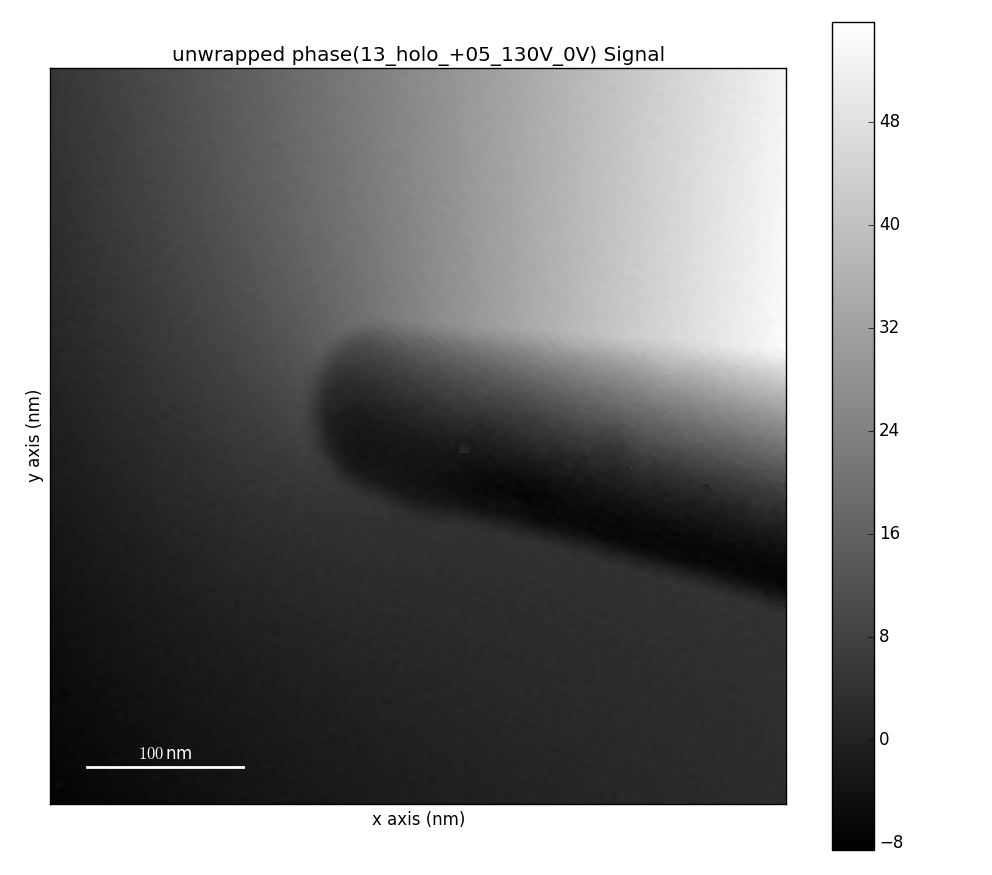
Unwrapped phase image.
Additionally, it is possible to change the smoothness of the sideband filter
edge (which is by default set to 5% of the filter radius) using parameter
sb_smoothness.
Both sb_size and sb_smoothness can be provided in desired units rather
than pixels (by default) by setting sb_unit value either to mrad or
nm for milliradians or inverse nanometers respectively. For example:
>>> wave_image = im.reconstruct_phase(reference_hologram,
...                                   sb_position=sb_position, sb_size=30,
...                                   sb_smoothness=0.05*30,sb_unit='mrad')
Also the reconstruct_phase()
method can output wave images with desired size (shape). By default the shape
of the original hologram is preserved. Though this leads to oversampling of the
output wave images, since the information is limited by the size of the
sideband filter. To avoid oversampling the output shape can be set to the
diameter of the sideband as follows:
>>> wave_image = im.reconstruct_phase(reference_hologram,
...                                   sb_position=sb_position,
...                                   sb_size=sb_sb_size,
...                                   output_shape=(2*sb_size, 2*sb_size))
Note that the
reconstruct_phase()
method can be called without parameters, which will cause their automatic
assignment by
estimate_sideband_position()
and estimate_sideband_size()
methods. This, however, is not recommended for not experienced users.
Getting hologram statistics
There are many reasons to have an access to some parameters of holograms which describe the quality of the data.
statistics() can be used to calculate carrier frequency,
fringe spacing and estimate fringe contrast. The method outputs dictionary with the values listed above calculated also
in different units. In particular fringe spacing is calculated in pixels (fringe sampling) as well as in
calibrated units. Carrier frequency is calculated in inverse pixels or calibrated units as well as radians.
Estimation of fringe contrast is either performed by division of standard deviation by mean value of hologram or
in Fourier space as twice the fraction of amplitude of sideband centre and amplitude of center band (i.e. FFT origin).
The first method is default and using it requires the fringe field to cover entire field of view; the method is
highly sensitive to any artifacts in holograms like dud pixels,
fresnel fringes and etc. The second method is less sensitive to the artifacts listed above and gives
reasonable estimation of fringe contrast even if the hologram is not covering entire field of view, but it is highly
sensitive to precise calculation of sideband position and therefore sometimes may underestimate the contrast.
The selection between to algorithms can be done using parameter fringe_contrast_algorithm setting it to
'statistical' or to 'fourier'. The side band position typically provided by a sb_position.
The statistics can be accessed as follows:
>>> statistics = im.statistics(sb_position=sb_position)
Note that by default the single_value parameter is True which forces the output of single values for each
entry of statistics dictionary calculated from first navigation pixel. (I.e. for image stacks only first image
will be used for calculating the statistics.) Otherwise:
>>> statistics = im.statistics(sb_position=sb_position, single_value=False)
Entries of statistics are Hyperspy signals containing the hologram parameters for each image in a stack.
The estimation of fringe spacing using 'fourier' method applies apodization in real space prior calculating FFT.
By default apodization parameter is set to hanning which applies Hanning window. Other options are using either
None or hamming for no apodization or Hamming window. Please note that for experimental conditions
especially with extreme sampling of fringes and strong contrast variation due to Fresnel effects
the calculated fringe contrast provides only an estimate and the values may differ strongly depending on apodization.
For further information see documentation of statistics().