Tools: the Signal class

The Signal class and its subclasses

Warning

This subsection can be a bit confusing for beginners. Do not worry if you do not understand it all.

HyperSpy stores the data in the BaseSignal class, that is the object that you get when e.g. you load a single file using load(). Most of the data analysis functions are also contained in this class or its specialized subclasses. The BaseSignal class contains general functionality that is available to all the subclasses. The subclasses provide functionality that is normally specific to a particular type of data, e.g. the Signal1D class provides common functionality to deal with one-dimensional (e.g. spectral) data and EELSSpectrum (which is a subclass of Signal1D) adds extra functionality to the Signal1D class for electron energy-loss spectroscopy data analysis.

The table below summarises all the currently available specialised BaseSignal subclasses.

The signals module, which contains all available signal subclasses, is imported in the user namespace when loading HyperSpy. In the following example we create a Signal2D instance from a 2D numpy array:

>>> im = hs.signals.Signal2D(np.random.random((64,64)))
>>> im
<Signal2D, title: , dimensions: (|64, 64)>

The different signals store other objects in what are called attributes. For examples, the data is stored in a numpy array in the data attribute, the original parameters in the original_metadata attribute, the mapped parameters in the metadata attribute and the axes information (including calibration) can be accessed (and modified) in the AxesManager attribute.

Signal initialization

Many of the values in the AxesManager can be set when making the BaseSignal object.

>>> dict0 = {'size': 10, 'name':'Axis0', 'units':'A', 'scale':0.2, 'offset':1}
>>> s = hs.signals.BaseSignal(np.random.random((10,20)), axes=[dict0, dict1])
>>> s.axes_manager
<Axes manager, axes: (|20, 10)>
            Name |   size |  index |  offset |   scale |  units
================ | ====== | ====== | ======= | ======= | ======
---------------- | ------ | ------ | ------- | ------- | ------
           Axis1 |     20 |        |       2 |     0.1 |      B
           Axis0 |     10 |        |       1 |     0.2 |      A

This also applies to the metadata.

>>> metadata_dict = {'General':{'name':'A BaseSignal'}}
>>> metadata_dict['General']['title'] = 'A BaseSignal title'
>>> s = hs.signals.BaseSignal(np.arange(10), metadata=metadata_dict)
>>> s.metadata
├── General
│   ├── name = A BaseSignal
│   └── title = A BaseSignal title
└── Signal
    ├── binned = False
    └── signal_type =

The navigation and signal dimensions

HyperSpy can deal with data of arbitrary dimensions. Each dimension is internally classified as either “navigation” or “signal” and the way this classification is done determines the behaviour of the signal.

The concept is probably best understood with an example: let’s imagine a three dimensional dataset e.g. a numpy array with dimensions (10, 20, 30). This dataset could be an spectrum image acquired by scanning over a sample in two dimensions. As in this case the signal is one-dimensional we use a Signal1D subclass for this data e.g.:

>>> s = hs.signals.Signal1D(np.random.random((10, 20, 30)))
>>> s
<Signal1D, title: , dimensions: (20, 10|30)>

In HyperSpy’s terminology, the signal dimension of this dataset is 30 and the navigation dimensions (20, 10). Notice the separator | between the navigation and signal dimensions.

However, the same dataset could also be interpreted as an image stack instead. Actually it could has been acquired by capturing two dimensional images at different wavelengths. Then it would be natural to identify the two spatial dimensions as the signal dimensions and the wavelength dimension as the navigation dimension. To view the data in this way we could have used a Signal2D instead e.g.:

>>> im = hs.signals.Signal2D(np.random.random((10, 20, 30)))
>>> im
<Signal2D, title: , dimensions: (10|30, 20)>

Indeed, for data analysis purposes, one may like to operate with an image stack as if it was a set of spectra or viceversa. One can easily switch between these two alternative ways of classifying the dimensions of a three-dimensional dataset by transforming between BaseSignal subclasses.

The same dataset could be seen as a three-dimensional signal:

>>> td = hs.signals.BaseSignal(np.random.random((10, 20, 30)))
>>> td
<BaseSignal, title: , dimensions: (|30, 20, 10)>

Notice that with use BaseSignal because there is no specialised subclass for three-dimensional data. Also note that by default BaseSignal interprets all dimensions as signal dimensions. We could also configure it to operate on the dataset as a three-dimensional array of scalars by changing the default view of BaseSignal by taking the transpose of it:

>>> scalar = td.T
>>> scalar
<BaseSignal, title: , dimensions: (30, 20, 10|)>

For more examples of manipulating signal axes in the “signal-navigation” space can be found in Transposing (changing signal spaces).

Note

Although each dimension can be arbitrarily classified as “navigation dimension” or “signal dimension”, for most common tasks there is no need to modify HyperSpy’s default choice.

Transforming between signal subclasses

The different subclasses are characterized by the signal_type metadata attribute, the data dtype and the signal dimension. See the table and diagram below. signal_type describes the nature of the signal. It can be any string, normally the acronym associated with a particular signal. In certain cases HyperSpy provides features that are only available for a particular signal type through BaseSignal subclasses. The BaseSignal method set_signal_type() changes the signal_type in place, which may result in a BaseSignal subclass transformation.

Furthermore, the dtype of the signal data also affects the subclass assignment. There are e.g. specialised signal subclasses to handle complex data (see the following diagram).

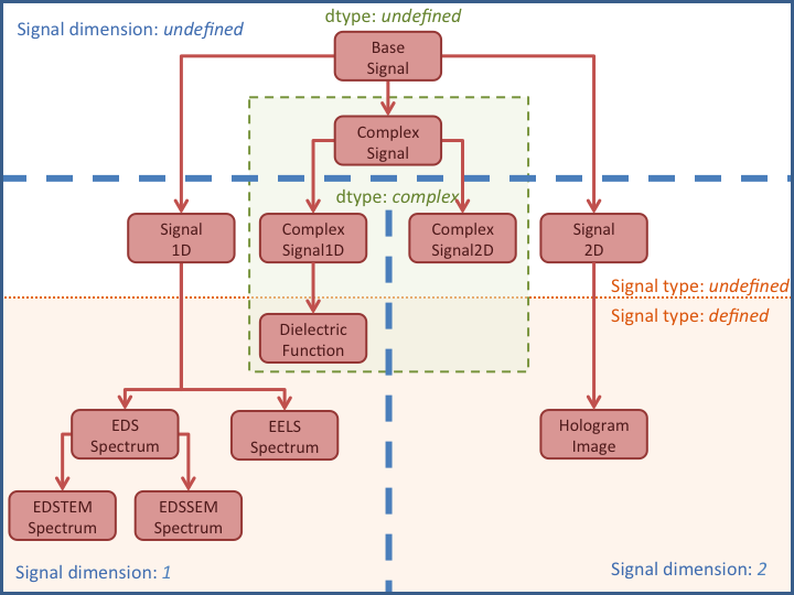
Diagram showing the inheritance structure of the different subclasses

BaseSignal subclass metadata attributes.

BaseSignal subclass	signal_dimension	signal_type	dtype
BaseSignal			real
Signal1D	1		real
EELSSpectrum	1	EELS	real
EDSSEMSpectrum	1	EDS_SEM	real
EDSTEM	1	EDS_TEM	real
Signal2D	2		real
HologramImage	2	hologram	real
DielectricFunction	1	DielectricFunction	complex
ComplexSignal			complex
ComplexSignal1D	1		complex
Complex2D	2		complex

The following example shows how to transform between different subclasses.

>>> s = hs.signals.Signal1D(np.random.random((10,20,100)))
>>> s
<Signal1D, title: , dimensions: (20, 10|100)>
>>> s.metadata
├── signal_type =
└── title =
>>> im = s.to_signal2D()
>>> im
<Signal2D, title: , dimensions: (100|20, 10)>
>>> im.metadata
├── signal_type =
└── title =
>>> s.set_signal_type("EELS")
>>> s
<EELSSpectrum, title: , dimensions: (20, 10|100)>
>>> s.change_dtype("complex")
>>> s
<ComplexSignal1D, title: , dimensions: (20, 10|100)>

Binned and unbinned signals

Signals that are a histogram of a probability density function (pdf) should have the signal.metadata.Signal.binned attribute set to True. This is because some methods operate differently in signals that are binned.

Changed in version 1.0: Simulation, SpectrumSimulation and ImageSimulation classes removed.

The default value of the binned attribute is shown in the following table:

Binned default values for the different subclasses.

BaseSignal subclass	binned
BaseSignal	False
Signal1D	False
EELSSpectrum	True
EDSSEMSpectrum	True
EDSTEM	True
Signal2D	False
ComplexSignal	False
ComplexSignal1D	False
Complex2Dmixin	False

To change the default value:

>>> s.metadata.Signal.binned = True

Generic tools

Below we briefly introduce some of the most commonly used tools (methods). For more details about a particular method click on its name. For a detailed list of all the methods available see the BaseSignal documentation.

The methods of this section are available to all the signals. In other chapters methods that are only available in specialized subclasses.

Mathematical operations

A number of mathematical operations are available in BaseSignal. Most of them are just wrapped numpy functions.

The methods that perform mathematical operation over one or more axis at a time are:

• sum()

• max()

• min()

• mean()

• std()

• var()

• nansum()

• nanmax()

• nanmin()

• nanmean()

• nanstd()

• nanvar()

Note that by default all this methods perform the operation over all navigation axes.

Example:

>>> s = hs.signals.BaseSignal(np.random.random((2,4,6)))
>>> s.axes_manager[0].name = 'E'
>>> s
<BaseSignal, title: , dimensions: (|6, 4, 2)>
>>> # by default perform operation over all navigation axes
>>> s.sum()
<BaseSignal, title: , dimensions: (|6, 4, 2)>
>>> # can also pass axes individually
>>> s.sum('E')
<Signal2D, title: , dimensions: (|4, 2)>
>>> # or a tuple of axes to operate on, with duplicates, by index or directly
>>> ans = s.sum((-1, s.axes_manager[1], 'E', 0))
>>> ans
<BaseSignal, title: , dimensions: (|1)>
>>> ans.axes_manager[0]
<Scalar axis, size: 1>

The following methods operate only on one axis at a time:

• diff()

• derivative()

• integrate_simpson()

• integrate1D()

• indexmin()

• indexmax()

• valuemin()

• valuemax()

All numpy ufunc can operate on BaseSignal instances, for example:

>>> s = hs.signals.Signal1D([0, 1])
>>> s.metadata.General.title = "A"
>>> s
<Signal1D, title: A, dimensions: (|2)>
>>> np.exp(s)
<Signal1D, title: exp(A), dimensions: (|2)>
>>> np.exp(s).data
array([ 1.        ,  2.71828183])
>>> np.power(s, 2)
<Signal1D, title: power(A, 2), dimensions: (|2)>
>>> np.add(s, s)
<Signal1D, title: add(A, A), dimensions: (|2)>
>>> np.add(hs.signals.Signal1D([0, 1]), hs.signals.Signal1D([0, 1]))
<Signal1D, title: add(Untitled Signal 1, Untitled Signal 2), dimensions: (|2)>

Notice that the title is automatically updated. When the signal has no title a new title is automatically generated:

>>> np.add(hs.signals.Signal1D([0, 1]), hs.signals.Signal1D([0, 1]))
<Signal1D, title: add(Untitled Signal 1, Untitled Signal 2), dimensions: (|2)>

Functions (other than unfucs) that operate on numpy arrays can also operate on BaseSignal instances, however they return a numpy array instead of a BaseSignal instance e.g.:

>>> np.angle(s)
array([ 0.,  0.])

Indexing

Indexing a BaseSignal provides a powerful, convenient and Pythonic way to access and modify its data. In HyperSpy indexing is achieved using isig and inav, which allow the navigation and signal dimensions to be indexed independently. The idea is essentially to specify a subset of the data based on its position in the array and it is therefore essential to know the convention adopted for specifying that position, which is described here.

Those new to Python may find indexing a somewhat esoteric concept but once mastered it is one of the most powerful features of Python based code and greatly simplifies many common tasks. HyperSpy’s Signal indexing is similar to numpy array indexing and those new to Python are encouraged to read the associated numpy documentation on the subject.

Key features of indexing in HyperSpy are as follows (note that some of these features differ from numpy):

• HyperSpy indexing does:

  • Allow independent indexing of signal and navigation dimensions

  • Support indexing with decimal numbers.

  • Support indexing with units.

  • Use the image order for indexing i.e. [x, y, z,…] (HyperSpy) vs […,z,y,x] (numpy)

• HyperSpy indexing does not:

  • Support indexing using arrays.

  • Allow the addition of new axes using the newaxis object.

The examples below illustrate a range of common indexing tasks.

First consider indexing a single spectrum, which has only one signal dimension (and no navigation dimensions) so we use isig:

>>> s = hs.signals.Signal1D(np.arange(10))
>>> s
<Signal1D, title: , dimensions: (|10)>
>>> s.data
array([0, 1, 2, 3, 4, 5, 6, 7, 8, 9])
>>> s.isig[0]
<Signal1D, title: , dimensions: (|1)>
>>> s.isig[0].data
array([0])
>>> s.isig[9].data
array([9])
>>> s.isig[-1].data
array([9])
>>> s.isig[:5]
<Signal1D, title: , dimensions: (|5)>
>>> s.isig[:5].data
array([0, 1, 2, 3, 4])
>>> s.isig[5::-1]
<Signal1D, title: , dimensions: (|6)>
>>> s.isig[5::-1]
<Signal1D, title: , dimensions: (|6)>
>>> s.isig[5::2]
<Signal1D, title: , dimensions: (|3)>
>>> s.isig[5::2].data
array([5, 7, 9])

Unlike numpy, HyperSpy supports indexing using decimal numbers or string (containing a decimal number and an units), in which case HyperSpy indexes using the axis scales instead of the indices.

>>> s = hs.signals.Signal1D(np.arange(10))
>>> s
<Signal1D, title: , dimensions: (|10)>
>>> s.data
array([0, 1, 2, 3, 4, 5, 6, 7, 8, 9])
>>> s.axes_manager[0].scale = 0.5
>>> s.axes_manager[0].axis
array([ 0. ,  0.5,  1. ,  1.5,  2. ,  2.5,  3. ,  3.5,  4. ,  4.5])
>>> s.isig[0.5:4.].data
array([1, 2, 3, 4, 5, 6, 7])
>>> s.isig[0.5:4].data
array([1, 2, 3])
>>> s.isig[0.5:4:2].data
array([1, 3])
>>> s.axes_manager[0].units = 'µm'
>>> s.isig[:'2000 nm'].data
array([0, 1, 2, 3])

Importantly the original BaseSignal and its “indexed self” share their data and, therefore, modifying the value of the data in one modifies the same value in the other. Note also that in the example below s.data is used to access the data as a numpy array directly and this array is then indexed using numpy indexing.

>>> s = hs.signals.Signal1D(np.arange(10))
>>> s
<Signal1D, title: , dimensions: (10,)>
>>> s.data
array([0, 1, 2, 3, 4, 5, 6, 7, 8, 9])
>>> si = s.isig[::2]
>>> si.data
array([0, 2, 4, 6, 8])
>>> si.data[:] = 10
>>> si.data
array([10, 10, 10, 10, 10])
>>> s.data
array([10,  1, 10,  3, 10,  5, 10,  7, 10,  9])
>>> s.data[:] = 0
>>> si.data
array([0, 0, 0, 0, 0])

Of course it is also possible to use the same syntax to index multidimensional data treating navigation axes using inav and signal axes using isig.

>>> s = hs.signals.Signal1D(np.arange(2*3*4).reshape((2,3,4)))
>>> s
<Signal1D, title: , dimensions: (3, 2|4)>
>>> s.data
array([[[ 0,  1,  2,  3],
    [ 4,  5,  6,  7],
    [ 8,  9, 10, 11]],

   [[12, 13, 14, 15],
    [16, 17, 18, 19],
    [20, 21, 22, 23]]])
>>> s.axes_manager[0].name = 'x'
>>> s.axes_manager[1].name = 'y'
>>> s.axes_manager[2].name = 't'
>>> s.axes_manager.signal_axes
(<t axis, size: 4>,)
>>> s.axes_manager.navigation_axes
(<x axis, size: 3, index: 0>, <y axis, size: 2, index: 0>)
>>> s.inav[0,0].data
array([0, 1, 2, 3])
>>> s.inav[0,0].axes_manager
<Axes manager, axes: (|4)>
            Name |   size |  index |  offset |   scale |  units
================ | ====== | ====== | ======= | ======= | ======
---------------- | ------ | ------ | ------- | ------- | ------
               t |      4 |        |       0 |       1 | <undefined>
>>> s.inav[0,0].isig[::-1].data
array([3, 2, 1, 0])
>>> s.isig[0]
<BaseSignal, title: , dimensions: (3, 2)>
>>> s.isig[0].axes_manager
<Axes manager, axes: (3, 2|)>
            Name |   size |  index |  offset |   scale |  units
================ | ====== | ====== | ======= | ======= | ======
               x |      3 |      0 |       0 |       1 | <undefined>
               y |      2 |      0 |       0 |       1 | <undefined>
---------------- | ------ | ------ | ------- | ------- | ------
>>> s.isig[0].data
array([[ 0,  4,  8],
   [12, 16, 20]])

Independent indexation of the signal and navigation dimensions is demonstrated further in the following:

>>> s = hs.signals.Signal1D(np.arange(2*3*4).reshape((2,3,4)))
>>> s
<Signal1D, title: , dimensions: (3, 2|4)>
>>> s.data
array([[[ 0,  1,  2,  3],
    [ 4,  5,  6,  7],
    [ 8,  9, 10, 11]],

   [[12, 13, 14, 15],
    [16, 17, 18, 19],
    [20, 21, 22, 23]]])
>>> s.axes_manager[0].name = 'x'
>>> s.axes_manager[1].name = 'y'
>>> s.axes_manager[2].name = 't'
>>> s.axes_manager.signal_axes
(<t axis, size: 4>,)
>>> s.axes_manager.navigation_axes
(<x axis, size: 3, index: 0>, <y axis, size: 2, index: 0>)
>>> s.inav[0,0].data
array([0, 1, 2, 3])
>>> s.inav[0,0].axes_manager
<Axes manager, axes: (|4)>
            Name |   size |  index |  offset |   scale |  units
================ | ====== | ====== | ======= | ======= | ======
---------------- | ------ | ------ | ------- | ------- | ------
               t |      4 |        |       0 |       1 | <undefined>
>>> s.isig[0]
<BaseSignal, title: , dimensions: (2, 3)>
>>> s.isig[0].axes_manager
<Axes manager, axes: (3, 2|)>
            Name |   size |  index |  offset |   scale |  units
================ | ====== | ====== | ======= | ======= | ======
               x |      3 |      0 |       0 |       1 | <undefined>
               y |      2 |      0 |       0 |       1 | <undefined>
---------------- | ------ | ------ | ------- | ------- | ------
>>> s.isig[0].data
array([[ 0,  4,  8],
   [12, 16, 20]])

The same syntax can be used to set the data values in signal and navigation dimensions respectively:

>>> s = hs.signals.Signal1D(np.arange(2*3*4).reshape((2,3,4)))
>>> s
<Signal1D, title: , dimensions: (3, 2|4)>
>>> s.data
array([[[ 0,  1,  2,  3],
    [ 4,  5,  6,  7],
    [ 8,  9, 10, 11]],

   [[12, 13, 14, 15],
    [16, 17, 18, 19],
    [20, 21, 22, 23]]])
>>> s.inav[0,0].data
array([0, 1, 2, 3])
>>> s.inav[0,0] = 1
>>> s.inav[0,0].data
array([1, 1, 1, 1])
>>> s.inav[0,0] = s.inav[1,1]
>>> s.inav[0,0].data
array([16, 17, 18, 19])

Signal operations

BaseSignal supports all the Python binary arithmetic operations (+, -, *, //, %, divmod(), pow(), **, <<, >>, &, ^, |), augmented binary assignments (+=, -=, *=, /=, //=, %=, **=, <<=, >>=, &=, ^=, |=), unary operations (-, +, abs() and ~) and rich comparisons operations (<, <=, ==, x!=y, <>, >, >=).

These operations are performed element-wise. When the dimensions of the signals are not equal numpy broadcasting rules apply independently for the navigation and signal axes.

Warning

Hyperspy does not check if the calibration of the signals matches.

In the following example s2 has only one navigation axis while s has two. However, because the size of their first navigation axis is the same, their dimensions are compatible and s2 is broadcasted to match s’s dimensions.

>>> s = hs.signals.Signal2D(np.ones((3,2,5,4)))
>>> s2 = hs.signals.Signal2D(np.ones((2,5,4)))
>>> s
<Signal2D, title: , dimensions: (2, 3|4, 5)>
>>> s2
<Signal2D, title: , dimensions: (2|4, 5)>
>>> s + s2
<Signal2D, title: , dimensions: (2, 3|4, 5)>

In the following example the dimensions are not compatible and an exception is raised.

>>> s = hs.signals.Signal2D(np.ones((3,2,5,4)))
>>> s2 = hs.signals.Signal2D(np.ones((3,5,4)))
>>> s
<Signal2D, title: , dimensions: (2, 3|4, 5)>
>>> s2
<Signal2D, title: , dimensions: (3|4, 5)>
>>> s + s2
Traceback (most recent call last):
  File "<ipython-input-55-044bb11a0bd9>", line 1, in <module>
    s + s2
  File "<string>", line 2, in __add__
  File "/home/fjd29/Python/hyperspy/hyperspy/signal.py", line 2686, in _binary_operator_ruler
    raise ValueError(exception_message)
ValueError: Invalid dimensions for this operation

Broadcasting operates exactly in the same way for the signal axes:

>>> s = hs.signals.Signal2D(np.ones((3,2,5,4)))
>>> s2 = hs.signals.Signal1D(np.ones((3, 2, 4)))
>>> s
<Signal2D, title: , dimensions: (2, 3|4, 5)>
>>> s2
<Signal1D, title: , dimensions: (2, 3|4)>
>>> s + s2
<Signal2D, title: , dimensions: (2, 3|4, 5)>

In-place operators also support broadcasting, but only when broadcasting would not change the left most signal dimensions:

>>> s += s2
>>> s
<Signal2D, title: , dimensions: (2, 3|4, 5)>
>>> s2 += s
Traceback (most recent call last):
  File "<ipython-input-64-fdb9d3a69771>", line 1, in <module>
    s2 += s
  File "<string>", line 2, in __iadd__
  File "/home/fjd29/Python/hyperspy/hyperspy/signal.py", line 2737, in _binary_operator_ruler
    self.data = getattr(sdata, op_name)(odata)
ValueError: non-broadcastable output operand with shape (3,2,1,4) doesn\'t match the broadcast shape (3,2,5,4)

Iterating over the navigation axes

BaseSignal instances are iterables over the navigation axes. For example, the following code creates a stack of 10 images and saves them in separate “png” files by iterating over the signal instance:

>>> image_stack = hs.signals.Signal2D(np.random.random((2, 5, 64,64)))
>>> for single_image in image_stack:
...    single_image.save("image %s.png" % str(image_stack.axes_manager.indices))
The "image (0, 0).png" file was created.
The "image (1, 0).png" file was created.
The "image (2, 0).png" file was created.
The "image (3, 0).png" file was created.
The "image (4, 0).png" file was created.
The "image (0, 1).png" file was created.
The "image (1, 1).png" file was created.
The "image (2, 1).png" file was created.
The "image (3, 1).png" file was created.
The "image (4, 1).png" file was created.

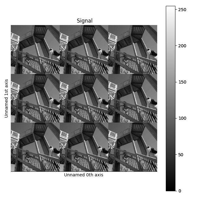
The data of the signal instance that is returned at each iteration is a view of the original data, a property that we can use to perform operations on the data. For example, the following code rotates the image at each coordinate by a given angle and uses the stack() function in combination with list comprehensions to make a horizontal “collage” of the image stack:

>>> import scipy.ndimage
>>> image_stack = hs.signals.Signal2D(np.array([scipy.misc.ascent()]*5))
>>> image_stack.axes_manager[1].name = "x"
>>> image_stack.axes_manager[2].name = "y"
>>> for image, angle in zip(image_stack, (0, 45, 90, 135, 180)):
...    image.data[:] = scipy.ndimage.rotate(image.data, angle=angle,
...    reshape=False)
>>> # clip data to integer range:
>>> image_stack.data = np.clip(image_stack.data, 0, 255)
>>> collage = hs.stack([image for image in image_stack], axis=0)
>>> collage.plot(scalebar=False)

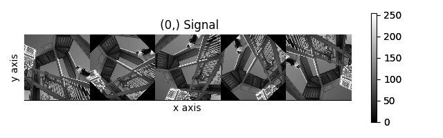
Rotation of images by iteration.

Iterating external functions with the map method

Performing an operation on the data at each coordinate, as in the previous example, using an external function can be more easily accomplished using the map() method:

>>> import scipy.ndimage
>>> image_stack = hs.signals.Signal2D(np.array([scipy.misc.ascent()]*4))
>>> image_stack.axes_manager[1].name = "x"
>>> image_stack.axes_manager[2].name = "y"
>>> image_stack.map(scipy.ndimage.rotate,
...                            angle=45,
...                            reshape=False)
>>> # clip data to integer range
>>> image_stack.data = np.clip(image_stack.data, 0, 255)
>>> collage = hs.stack([image for image in image_stack], axis=0)
>>> collage.plot()

Rotation of images by the same amount using map().

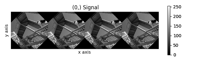
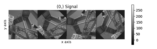
The map() method can also take variable arguments as in the following example.

>>> import scipy.ndimage
>>> image_stack = hs.signals.Signal2D(np.array([scipy.misc.ascent()]*4))
>>> image_stack.axes_manager[1].name = "x"
>>> image_stack.axes_manager[2].name = "y"
>>> angles = hs.signals.BaseSignal(np.array([0, 45, 90, 135]))
>>> image_stack.map(scipy.ndimage.rotate,
...                            angle=angles.T,
...                            reshape=False)

Rotation of images using map() with different arguments for each image in the stack.

New in version 1.2.0: inplace keyword and non-preserved output shapes

If all function calls do not return identically-shaped results, only navigation information is preserved, and the final result is an array where each element corresponds to the result of the function (or arbitrary object type). As such, most HyperSpy functions cannot operate on such Signal, and the data should be accessed directly.

inplace keyword (by default True) of the map() method allows either overwriting the current data (default, True) or storing it to a new signal (False).

>>> import scipy.ndimage
>>> image_stack = hs.signals.Signal2D(np.array([scipy.misc.ascent()]*4))
>>> angles = hs.signals.BaseSignal(np.array([0, 45, 90, 135]))
>>> result = image_stack.map(scipy.ndimage.rotate,
...                            angle=angles.T,
...                            inplace=False,
...                            reshape=True)
100%|████████████████████████████████████████████| 4/4 [00:00<00:00, 18.42it/s]

>>> result
<BaseSignal, title: , dimensions: (4|)>
>>> image_stack.data.dtype
dtype('O')
>>> for d in result.data.flat:
...     print(d.shape)
(512, 512)
(724, 724)
(512, 512)
(724, 724)

New in version 1.2.0: parallel keyword.

The execution can be sped up by passing parallel keyword to the map() method:

>>> import time
>>> def slow_func(data):
...     time.sleep(1.)
...     return data + 1
>>> s = hs.signals.Signal1D(np.arange(20).reshape((20,1)))
>>> s
<Signal1D, title: , dimensions: (20|1)>
>>> s.map(slow_func, parallel=False)
100%|██████████████████████████████████████| 20/20 [00:20<00:00,  1.00s/it]
>>> # some operations will be done in parallel:
>>> s.map(slow_func, parallel=True)
100%|██████████████████████████████████████| 20/20 [00:02<00:00,  6.73it/s]

New in version 1.4: Iterating over signal using a parameter with no navigation dimension.

In this case, the parameter is cyclically iterated over the navigation dimension of the input signal. In the example below, signal s is multiplied by a cosine parameter d, which is repeated over the navigation dimension of s.

>>> s = hs.signals.Signal1D(np.random.rand(10, 512))
>>> d = hs.signals.Signal1D(np.cos(np.linspace(0., 2*np.pi, 512)))
>>> s.map(lambda A, B: A * B, B=d)
100%|██████████| 10/10 [00:00<00:00, 2573.19it/s]

Cropping

Cropping can be performed in a very compact and powerful way using Indexing . In addition it can be performed using the following method or GUIs if cropping signal1D or signal2D. There is also a general crop() method that operates in place.

Rebinning

New in version 1.3: rebin() generalized to remove the constrain of the new_shape needing to be a divisor of data.shape.

The rebin() methods supports rebinning the data to arbitrary new shapes as long as the number of dimensions stays the same. However, internally, it uses two different algorithms to perform the task. Only when the new shape dimensions are divisors of the old shape’s, the operation supports lazy-evaluation and is usually faster. Otherwise, the operation requires linear interpolation and is generally slower if Numba is not installed.

For example, the following two equivalent rebinning operations can be performed lazily:

>>> s = hs.datasets.example_signals.EDS_SEM_Spectrum().as_lazy()
>>> print(s)
<LazyEDSSEMSpectrum, title: EDS SEM Spectrum, dimensions: (|1024)>
>>> print(s.rebin(scale=[2]))
<LazyEDSSEMSpectrum, title: EDS SEM Spectrum, dimensions: (|512)>

>>> s = hs.datasets.example_signals.EDS_SEM_Spectrum().as_lazy()
>>> print(s.rebin(new_shape=[512]))
<LazyEDSSEMSpectrum, title: EDS SEM Spectrum, dimensions: (|512)>

On the other hand, the following rebinning operation requires interpolation and cannot be performed lazily:

>>> spectrum = hs.signals.EDSTEMSpectrum(np.ones([4, 4, 10]))
>>> spectrum.data[1, 2, 9] = 5
>>> print(spectrum)
<EDSTEMSpectrum, title: , dimensions: (4, 4|10)>
>>> print ('Sum = ', spectrum.data.sum())
Sum =  164.0
>>> scale = [0.5, 0.5, 5]
>>> test = spectrum.rebin(scale=scale)
>>> test2 = spectrum.rebin(new_shape=(8, 8, 2)) # Equivalent to the above
>>> print(test)
<EDSTEMSpectrum, title: , dimensions: (8, 8|2)>
>>> print(test2)
<EDSTEMSpectrum, title: , dimensions: (8, 8|2)>
>>> print('Sum =', test.data.sum())
Sum = 164.0
>>> print('Sum =', test2.data.sum())
Sum = 164.0
>>> spectrum.as_lazy().rebin(scale=scale)
Traceback (most recent call last):
  File "<ipython-input-26-49bca19ebf34>", line 1, in <module>
    spectrum.as_lazy().rebin(scale=scale)
  File "/home/fjd29/Python/hyperspy3/hyperspy/_signals/eds.py", line 184, in rebin
    m = super().rebin(new_shape=new_shape, scale=scale, crop=crop, out=out)
  File "/home/fjd29/Python/hyperspy3/hyperspy/_signals/lazy.py", line 246, in rebin
    "Lazy rebin requires scale to be integer and divisor of the "
NotImplementedError: Lazy rebin requires scale to be integer and divisor of the original signal shape

Folding and unfolding

When dealing with multidimensional datasets it is sometimes useful to transform the data into a two dimensional dataset. This can be accomplished using the following two methods:

• fold()

• unfold()

It is also possible to unfold only the navigation or only the signal space:

• unfold_navigation_space()

• unfold_signal_space()

Splitting and stacking

Several objects can be stacked together over an existing axis or over a new axis using the stack() function, if they share axis with same dimension.

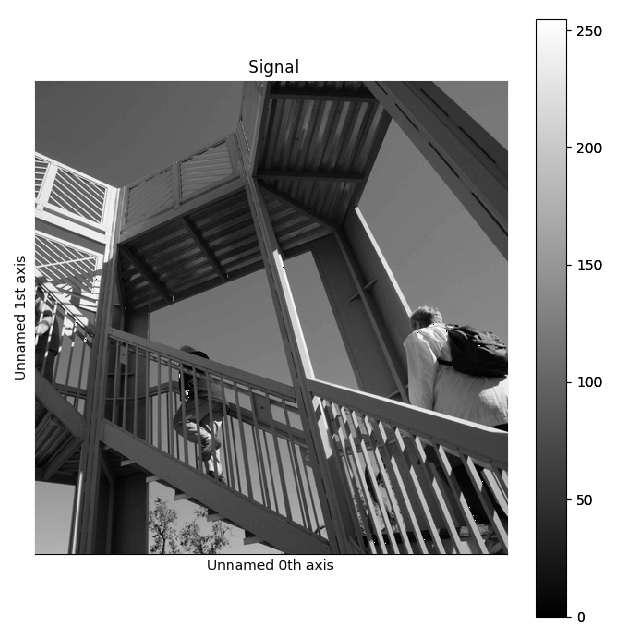
>>> image = hs.signals.Signal2D(scipy.misc.ascent())
>>> image = hs.stack([hs.stack([image]*3,axis=0)]*3,axis=1)
>>> image.plot()

Stacking example.

An object can be split into several objects with the split() method. This function can be used to reverse the stack() function:

>>> image = image.split()[0].split()[0]
>>> image.plot()

Splitting example.

FFT and iFFT

New in version 1.4: fft() and ifft() method and fft_shift and power_spectrum plot keyword arguments.

The Fast Fourier transform and its inverse can be applied on a signal with the fft() and the ifft() methods.

>>> im = hs.datasets.example_signals.object_hologram()
>>> im.fft().plot()

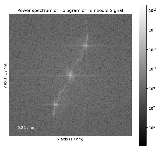
Note that for visual inspection of FFT, it is common to plot the power spectrum (absolute value of the complex signal) on a logarithmic scale rather than the FFT itself as it is done in the example above. By default, in case of FFT, HyperSpy plots the power spectrum and shifts the zero frequency component to the center of the signal. This can be changed by setting power_spectrum=False and fft_shift=False parameters of the plot method.

By default, both methods calculate FFT and IFFT with origin at (0, 0) (not in the centre of FFT). Use fft_shift=True option to calculate FFT and the inverse with origin shifted in the centre. ROIs doesn’t work when the FFT is plotted with fft_shift=True.

>>> im_ifft = im.fft(fft_shift=True).ifft(fft_shift=True)

Changing the data type

Even if the original data is recorded with a limited dynamic range, it is often desirable to perform the analysis operations with a higher precision. Conversely, if space is limited, storing in a shorter data type can decrease the file size. The change_dtype() changes the data type in place, e.g.:

>>> s = hs.load('EELS Signal1D Signal2D (high-loss).dm3')
    Title: EELS Signal1D Signal2D (high-loss).dm3
    Signal type: EELS
    Data dimensions: (21, 42, 2048)
    Data representation: spectrum
    Data type: float32
>>> s.change_dtype('float64')
>>> print(s)
    Title: EELS Signal1D Signal2D (high-loss).dm3
    Signal type: EELS
    Data dimensions: (21, 42, 2048)
    Data representation: spectrum
    Data type: float64

In addition to all standard numpy dtypes, HyperSpy supports four extra dtypes for RGB images for visualization purposes only: rgb8, rgba8, rgb16 and rgba16. This includes of course multi-dimensional RGB images.

The requirements for changing from and to any rgbx dtype are more strict than for most other dtype conversions. To change to a rgbx dtype the signal_dimension must be 1 and its size 3 (4) 3(4) for rgb (or rgba) dtypes and the dtype must be uint8 (uint16) for rgbx8 (rgbx16). After conversion the signal_dimension becomes 2.

Most operations on signals with RGB dtypes will fail. For processing simply change their dtype to uint8 (uint16).The dtype of images of dtype rgbx8 (rgbx16) can only be changed to uint8 (uint16) and the signal_dimension becomes 1.

In the following example we create a 1D signal with signal size 3 and with dtype uint16 and change its dtype to rgb16 for plotting.

>>> rgb_test = np.zeros((1024, 1024, 3))
>>> ly, lx = rgb_test.shape[:2]
>>> offset_factor = 0.16
>>> size_factor = 3
>>> Y, X = np.ogrid[0:lx, 0:ly]
>>> rgb_test[:,:,0] = (X - lx / 2 - lx*offset_factor) ** 2 + \
...                   (Y - ly / 2 - ly*offset_factor) ** 2 < \
...                   lx * ly / size_factor **2
>>> rgb_test[:,:,1] = (X - lx / 2 + lx*offset_factor) ** 2 + \
...                   (Y - ly / 2 - ly*offset_factor) ** 2 < \
...                   lx * ly / size_factor **2
>>> rgb_test[:,:,2] = (X - lx / 2) ** 2 + \
...                   (Y - ly / 2 + ly*offset_factor) ** 2 \
...                   < lx * ly / size_factor **2
>>> rgb_test *= 2**16 - 1
>>> s = hs.signals.Signal1D(rgb_test)
>>> s.change_dtype("uint16")
>>> s
<Signal1D, title: , dimensions: (1024, 1024|3)>
>>> s.change_dtype("rgb16")
>>> s
<Signal2D, title: , dimensions: (|1024, 1024)>
>>> s.plot()

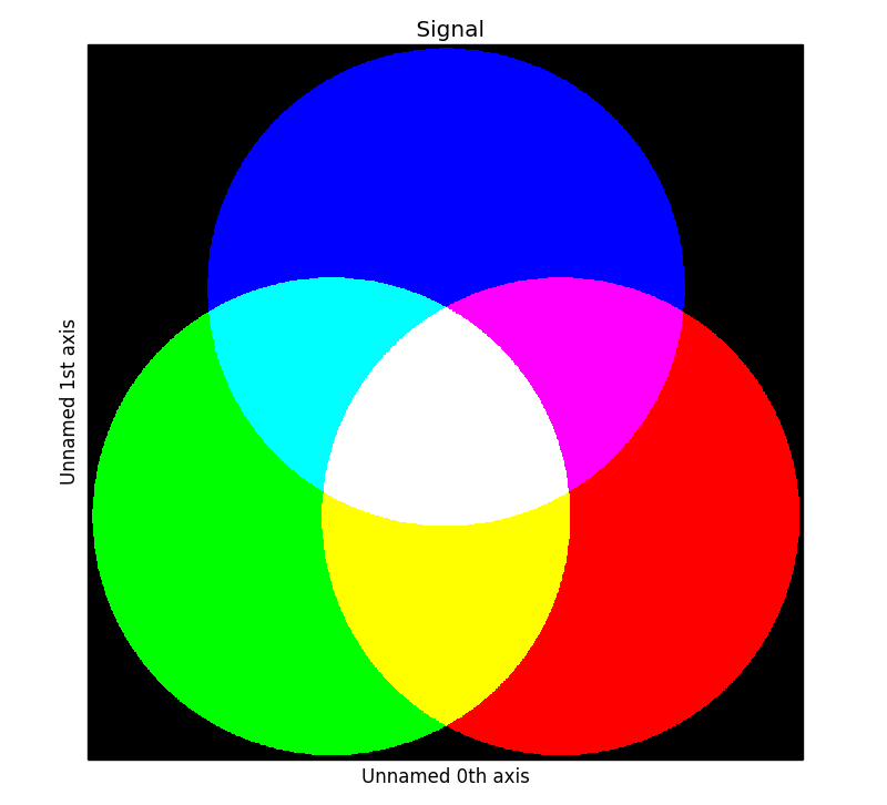
RGB data type example.

Transposing (changing signal spaces)

New in version 1.1.

transpose() method changes how the dataset dimensions are interpreted (as signal or navigation axes). By default is swaps the signal and navigation axes. For example:

>>> s = hs.signals.Signal1D(np.zeros((4,5,6)))
>>> s
<Signal1D, title: , dimensions: (5, 4|6)>
>>> s.transpose()
<Signal2D, title: , dimensions: (6|4, 5)>

For T() is a shortcut for the default behaviour:

>>> s = hs.signals.Signal1D(np.zeros((4,5,6))).T
<Signal2D, title: , dimensions: (6|4, 5)>

The method accepts both explicit axes to keep in either space, or just a number of axes required in one space (just one number can be specified, as the other is defined as “all other axes”). When axes order is not explicitly defined, they are “rolled” from one space to the other as if the <navigation axes | signal axes > wrap a circle. The example below should help clarifying this.

>>> # just create a signal with many distinct dimensions
>>> s = hs.signals.BaseSignal(np.random.rand(1,2,3,4,5,6,7,8,9))
>>> s
<BaseSignal, title: , dimensions: (|9, 8, 7, 6, 5, 4, 3, 2, 1)>
>>> s.transpose(signal_axes=5) # roll to leave 5 axes in signal space
<BaseSignal, title: , dimensions: (4, 3, 2, 1|9, 8, 7, 6, 5)>
>>> s.transpose(navigation_axes=3) # roll leave 3 axes in navigation space
<BaseSignal, title: , dimensions: (3, 2, 1|9, 8, 7, 6, 5, 4)>
>>> # 3 explicitly defined axes in signal space
>>> s.transpose(signal_axes=[0, 2, 6])
<BaseSignal, title: , dimensions: (8, 6, 5, 4, 2, 1|9, 7, 3)>
>>> # A mix of two lists, but specifying all axes explicitly
>>> # The order of axes is preserved in both lists
>>> s.transpose(navigation_axes=[1, 2, 3, 4, 5, 8], signal_axes=[0, 6, 7])
<BaseSignal, title: , dimensions: (8, 7, 6, 5, 4, 1|9, 3, 2)>

A convenience functions transpose() is available to operate on many signals at once, for example enabling plotting any-dimension signals trivially:

>>> s2 = hs.signals.BaseSignal(np.random.rand(2, 2)) # 2D signal
>>> s3 = hs.signals.BaseSignal(np.random.rand(3, 3, 3)) # 3D signal
>>> s4 = hs.signals.BaseSignal(np.random.rand(4, 4, 4, 4)) # 4D signal
>>> hs.plot.plot_images(hs.transpose(s2, s3, s4, signal_axes=2))

The transpose() method accepts keyword argument optimize, which is False by default, meaning modifying the output signal data always modifies the original data i.e. the data is just a view of the original data. If True, the method ensures the data in memory is stored in the most efficient manner for iterating by making a copy of the data if required, hence modifying the output signal data not always modifies the original data.

The convenience methods as_signal1D() and as_signal2D() internally use transpose(), but always optimize the data for iteration over the navigation axes if required. Hence, these methods do not always return a view of the original data. If a copy of the data is required use deepcopy() on the output of any of these methods e.g.:

>>> hs.signals.Signal1D(np.zeros((4,5,6))).T.deepcopy()
<Signal2D, title: , dimensions: (6|4, 5)>

Basic statistical analysis

get_histogram() computes the histogram and conveniently returns it as signal instance. It provides methods to calculate the bins. print_summary_statistics() prints the five-number summary statistics of the data.

These two methods can be combined with get_current_signal() to compute the histogram or print the summary statistics of the signal at the current coordinates, e.g:

>>> s = hs.signals.EELSSpectrum(np.random.normal(size=(10,100)))
>>> s.print_summary_statistics()
Summary statistics
------------------
mean:       0.021
std:        0.957
min:        -3.991
Q1: -0.608
median:     0.013
Q3: 0.652
max:        2.751

>>> s.get_current_signal().print_summary_statistics()
Summary statistics
------------------
mean:   -0.019
std:    0.855
min:    -2.803
Q1: -0.451
median: -0.038
Q3: 0.484
max:    1.992

Histogram of different objects can be compared with the functions plot_histograms() (see visualisation for the plotting options). For example, with histograms of several random chi-square distributions:

>>> img = hs.signals.Signal2D([np.random.chisquare(i+1,[100,100]) for
...                            i in range(5)])
>>> hs.plot.plot_histograms(img,legend='auto')

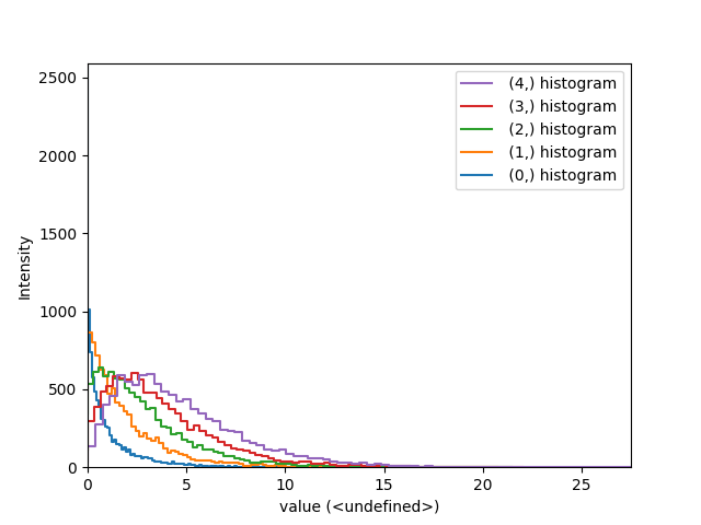
Comparing histograms.

Setting the noise properties

Some data operations require the data variance. Those methods use the metadata.Signal.Noise_properties.variance attribute if it exists. You can set this attribute as in the following example where we set the variance to be 10:

s.metadata.Signal.set_item("Noise_properties.variance", 10)

For heterocedastic noise the variance attribute must be a BaseSignal. Poissonian noise is a common case of heterocedastic noise where the variance is equal to the expected value. The estimate_poissonian_noise_variance() BaseSignal method can help setting the variance of data with semi-poissonian noise. With the default arguments, this method simply sets the variance attribute to the given expected_value. However, more generally (although then noise is not strictly poissonian), the variance may be proportional to the expected value. Moreover, when the noise is a mixture of white (gaussian) and poissonian noise, the variance is described by the following linear model:

Where a is the gain_factor, b is the gain_offset (the Gaussian noise variance) and c the correlation_factor. The correlation factor accounts for correlation of adjacent signal elements that can be modelled as a convolution with a Gaussian point spread function. estimate_poissonian_noise_variance() can be used to set the noise properties when the variance can be described by this linear model, for example:

>>> s = hs.signals.Spectrum(np.ones(100))
>>> s.add_poissonian_noise()
>>> s.metadata
├── General
│   └── title =
└── Signal
    ├── binned = False
    └── signal_type =

>>> s.estimate_poissonian_noise_variance()
>>> s.metadata
├── General
│   └── title =
└── Signal
    ├── Noise_properties
    │   ├── Variance_linear_model
    │   │   ├── correlation_factor = 1
    │   │   ├── gain_factor = 1
    │   │   └── gain_offset = 0
    │   └── variance = <SpectrumSimulation, title: Variance of , dimensions: (|100)>
    ├── binned = False
    └── signal_type =

Speeding up operations

Reusing a Signal for output

Many signal methods create and return a new signal. For fast operations, the new signal creation time is non-negligible. Also, when the operation is repeated many times, for example in a loop, the cumulative creation time can become significant. Therefore, many operations on BaseSignal accept an optional argument out. If an existing signal is passed to out, the function output will be placed into that signal, instead of being returned in a new signal. The following example shows how to use this feature to slice a BaseSignal. It is important to know that the BaseSignal instance passed in the out argument must be well-suited for the purpose. Often this means that it must have the same axes and data shape as the BaseSignal that would normally be returned by the operation.

>>> s = hs.signals.Signal1D(np.arange(10))
>>> s_sum = s.sum(0)
>>> s_sum.data
array([45])
>>> s.isig[:5].sum(0, out=s_sum)
>>> s_sum.data
array([10])
>>> s_roi = s.isig[:3]
>>> s_roi
<Signal1D, title: , dimensions: (|3)>
>>> s.isig.__getitem__(slice(None, 5), out=s_roi)
>>> s_roi
<Signal1D, title: , dimensions: (|5)>

Interactive operations

The function interactive() ease the task of defining operations that are automatically updated when an event is triggered. By default it recomputes the operation when data or the axes of the original signal changes.

>>> s = hs.signals.Signal1D(np.arange(10.))
>>> ssum = hs.interactive(s.sum, axis=0)
>>> ssum.data
array([45.0])
>>> s.data /= 10
>>> s.events.data_changed.trigger(s)
>>> ssum.data
array([ 4.5])

The interactive operations can be chained.

>>> s = hs.signals.Signal1D(np.arange(2 * 3 * 4).reshape((2, 3, 4)))
>>> ssum = hs.interactive(s.sum, axis=0)
>>> ssum_mean = hs.interactive(ssum.mean, axis=0)
>>> ssum_mean.data
array([ 30.,  33.,  36.,  39.])
>>> s.data
array([[[ 0,  1,  2,  3],
        [ 4,  5,  6,  7],
        [ 8,  9, 10, 11]],

       [[12, 13, 14, 15],
        [16, 17, 18, 19],
        [20, 21, 22, 23]]])
>>> s.data *= 10
>>> s.events.data_changed.trigger(obj=s)
>>> ssum_mean.data
array([ 300.,  330.,  360.,  390.])

Region Of Interest (ROI)

A number of different ROIs are available:

• Point1DROI

• Point2DROI

• SpanROI

• RectangularROI

• CircleROI

• Line2DROI

Once created, a ROI can be used to return a part of any compatible signal:

>>> s = hs.signals.Signal1D(np.arange(2000).reshape((20,10,10)))
>>> im = hs.signals.Signal2D(np.arange(100).reshape((10,10)))
>>> roi = hs.roi.RectangularROI(left=3, right=7, top=2, bottom=5)
>>> sr = roi(s)
>>> sr
<Signal1D, title: , dimensions: (4, 3|10)>
>>> imr = roi(im)
>>> imr
<Signal2D, title: , dimensions: (|4, 3)>

ROIs can also be used interactively with widgets. The following examples shows how to interactively apply ROIs to an image. Note that it is necessary to plot the signal onto which the widgets will be added before calling interactive().

>>> import scipy.misc
>>> im = hs.signals.Signal2D(scipy.misc.ascent())
>>> rectangular_roi = hs.roi.RectangularROI(left=30, right=500,
...                                         top=200, bottom=400)
>>> line_roi = hs.roi.Line2DROI(0, 0, 512, 512, 1)
>>> point_roi = hs.roi.Point2DROI(256, 256)
>>> im.plot()
>>> roi2D = rectangular_roi.interactive(im, color="blue")
>>> roi1D = line_roi.interactive(im, color="yellow")
>>> roi0D = point_roi.interactive(im, color="red")

Notably, since ROIs are independent from the signals they sub-select, the widget can be plotted on a different signal altogether.

>>> import scipy.misc
>>> im = hs.signals.Signal2D(scipy.misc.ascent())
>>> s = hs.signals.Signal1D(np.random.rand(512, 512, 512))
>>> roi = hs.roi.RectangularROI(left=30, right=77, top=20, bottom=50)
>>> s.plot() # plot signal to have where to display the widget
>>> imr = roi.interactive(im, navigation_signal=s, color="red")
>>> roi(im).plot()

ROIs are implemented in terms of physical coordinates and not pixels, so with proper calibration will always point to the same region.

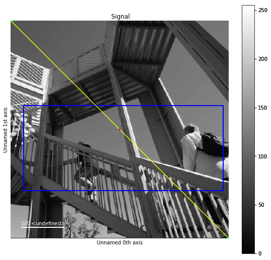
And of course, as all interactive operations, interactive ROIs are chainable. The following example shows how to display interactively the histogram of a rectangular ROI. Notice how we customise the default event connections in order to increase responsiveness.

>>> import scipy.misc
>>> im = hs.signals.Signal2D(scipy.misc.ascent())
>>> im.plot()
>>> roi = hs.roi.RectangularROI(left=30, right=500, top=200, bottom=400)
>>> im_roi = roi.interactive(im, color="red")
>>> roi_hist =hs.interactive(im_roi.get_histogram,
...                          event=im_roi.axes_manager.events.\
...                                any_axis_changed,
...                          recompute_out_event=None)
>>> roi_hist.plot()

New in version 1.3: ROIs can be used in place of slices when indexing and to define a signal range in functions taken a signal_range argument.

ROIs can be used in place of slices when indexing and to define a signal range in functions taken a signal_range argument. For example:

>>> s = hs.datasets.example_signals.EDS_TEM_Spectrum()
>>> roi = hs.roi.SpanROI(left=5, right=15)
>>> sc = s.isig[roi]
>>> s.remove_background(signal_range=roi, background_type="Polynomial")
>>> im = hs.datasets.example_signals.object_hologram()
>>> roi = hs.roi.RectangularROI(left=120, right=460., top=300, bottom=560)
>>> imc = im.isig[roi]

New in version 1.3: gui() method.

All ROIs have a gui() method that displays an user interface if a hyperspy GUI is installed (currently only works with the hyperspy_gui_ipywidgets GUI), enabling precise control of the ROI parameters:

>>> # continuing from above:
>>> roi.gui()

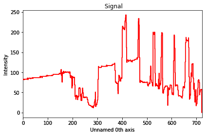
New in version 1.4: angle() can be used to calculate an angle between ROI line and one of the axes providing its name through optional argument axis:

>>> import scipy
>>> holo = hs.datasets.example_signals.object_hologram()
>>> roi = hs.roi.Line2DROI(x1=465.577, y1=445.15, x2=169.4, y2=387.731, linewidth=0)
>>> holo.plot()
>>> ss = roi.interactive(holo)

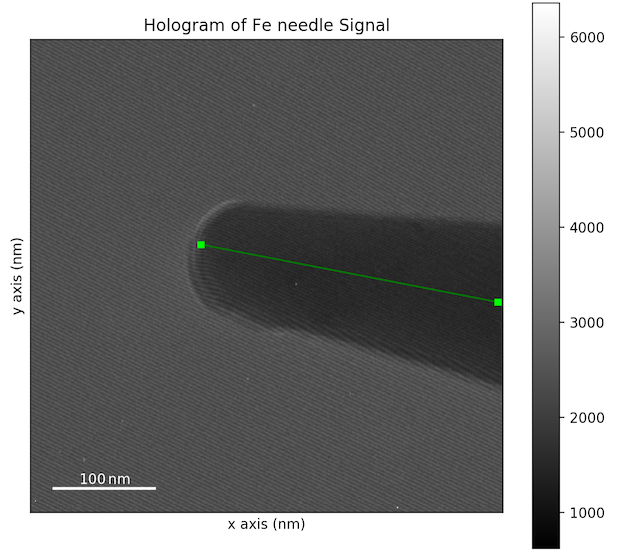
>>> roi.angle(axis='y')
-100.97166759025453

By default output of the method is in degrees, though radians can be selected as follows:

>>> roi.angle(axis='vertical', units='radians')
-1.7622880506791903

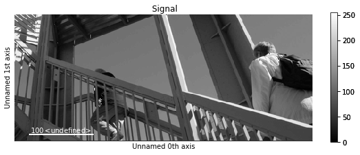
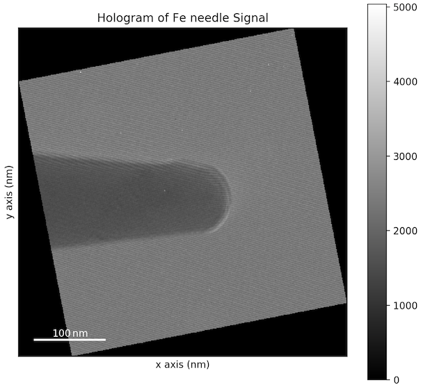
Conveniently, angle() can be used to rotate image to align selected features with respect to vertical or horizontal axis:

>>> holo.map(scipy.ndimage.rotate, angle=roi.angle(axis='horizontal'), inplace=False).plot()

Handling complex data

The HyperSpy ComplexSignal signal class and its subclasses for 1-dimensional and 2-dimensional data allow the user to access complex properties like the real and imag parts of the data or the amplitude (also known as the modulus) and phase (also known as angle or argument) directly. Getting and setting those properties can be done as follows:

>>> real = s.real      # real is a new HS signal accessing the same data
>>> s.real = new_real  # new_real can be an array or signal
>>> imag = s.imag      # imag  is a new HS signal accessing the same data
>>> s.imag = new_imag  # new_imag can be an array or signal

It is important to note that data passed to the constructor of a ComplexSignal (or to a subclass), which is not already complex, will be converted to the numpy standard of np.complex/np.complex128. data which is already complex will be passed as is.

To transform a real signal into a complex one use:

>>> s.change_dtype(complex)

Changing the dtype of a complex signal to something real is not clearly defined and thus not directly possible. Use the real, imag, amplitude or phase properties instead to extract the real data that is desired.

Calculate the angle / phase / argument

The angle() function can be used to calculate the angle, which is equivalent to using the phase property if no argument is used. If the data is real, the angle will be 0 for positive values and 2$pi$ for negative values. If the deg parameter is set to True, the result will be given in degrees, otherwise in rad (default). The underlying function is the angle() function. angle() will return an appropriate HyperSpy signal.

Phase unwrapping

With the unwrapped_phase() method the complex phase of a signal can be unwrapped and returned as a new signal. The underlying method is unwrap(), which uses the algorithm described in [Herraez].

Add a linear phase ramp

For 2-dimensional complex images, a linear phase ramp can be added to the signal via the add_phase_ramp() method. The parameters ramp_x and ramp_y dictate the slope of the ramp in x- and y direction, while the offset is determined by the offset parameter. The fulcrum of the linear ramp is at the origin and the slopes are given in units of the axis with the according scale taken into account. Both are available via the AxesManager of the signal.