Getting started
Starting Python in Windows
If you used the bundle installation you should be able to use the context menus to get started. Right-click on the folder containing the data you wish to analyse and select “Jupyter notebook here” or “Jupyter qtconsole here”. We recommend the former, since notebooks have many advantages over conventional consoles, as will be illustrated in later sections. The examples in some later sections assume Notebook operation. A new tab should appear in your default browser listing the files in the selected folder. To start a python notebook choose “Python 3” in the “New” drop-down menu at the top right of the page. Another new tab will open which is your Notebook.
Starting Python in Linux and MacOS
You can start IPython by opening a system terminal and executing ipython,
(optionally followed by the “frontend”: “qtconsole” for example). However, in
most cases, the most agreeable way to work with HyperSpy interactively
is using the Jupyter Notebook (previously known as
the IPython Notebook), which can be started as follows:
$ jupyter notebook
Linux users may find it more convenient to start Jupyter/IPython from the file manager context menu. In either OS you can also start by double-clicking a notebook file if one already exists.
Starting HyperSpy in the notebook (or terminal)
Typically you will need to set up IPython for interactive plotting with
matplotlib using
%matplotlib (which is known as a ‘Jupyter magic’)
before executing any plotting command. So, typically, after starting
IPython, you can import HyperSpy and set up interactive matplotlib plotting by
executing the following two lines in the IPython terminal (In these docs we
normally use the general Python prompt symbol >>> but you will probably
see In [1]: etc.):
>>> %matplotlib qt
>>> import hyperspy.api as hs
Note that to execute lines of code in the notebook you must press
Shift+Return. (For details about notebooks and their functionality try
the help menu in the notebook). Next, import two useful modules: numpy and
matplotlib.pyplot, as follows:
>>> import numpy as np
>>> import matplotlib.pyplot as plt
The rest of the documentation will assume you have done this. It also assumes that you have installed at least one of HyperSpy’s GUI packages: jupyter widgets GUI and the traitsui GUI.
By default, HyperSpy warns the user if one of the GUI packages is not installed.
These warnings can be turned off using the
Preferences GUI
(see here for more information) or
programmatically as follows:
>>> import hyperspy.api as hs
>>> hs.preferences.GUIs.warn_if_guis_are_missing = False
>>> hs.preferences.save()
Now you are ready to load your data (see below).
Changed in version v1.3: HyperSpy works with all matplotlib backends, including the nbagg backend that enables interactive plotting embedded in the jupyter notebook.
Warning
When using the qt4 backend in Python 2 the matplotlib magic must be executed after importing HyperSpy and qt must be the default HyperSpy backend.
Note
When running in a headless system it is necessary to set the matplotlib backend appropiately to avoid a cannot connect to X server error, for example as follows:
>>> import matplotlib
>>> matplotlib.rcParams["backend"] = "Agg"
>>> import hyperspy.api as hs
Getting help
When using IPython, the documentation (docstring in Python jargon) can be accessed by adding a question mark to the name of a function. e.g.:
>>> hs?
>>> hs.load?
>>> hs.signals?
This syntax is a shortcut to the standard way one of displaying the help associated to a given functions (docstring in Python jargon) and it is one of the many features of IPython, which is the interactive python shell that HyperSpy uses under the hood.
Please note that the documentation of the code is a work in progress, so not all the objects are documented yet.
Up-to-date documentation is always available in the HyperSpy website.
Autocompletion
Another useful IPython feature is the autocompletion of commands and filenames using the tab and arrow keys. It is highly recommended to read the Ipython documentation (specially their Getting started section) for many more useful features that will boost your efficiency when working with HyperSpy/Python interactively.
Loading data
Once HyperSpy is running, to load from a supported file format (see Supported formats) simply type:
>>> s = hs.load("filename")
Hint
The load function returns an object that contains data read from the file.
We assign this object to the variable s but you can choose any (valid)
variable name you like. for the filename, don’t forget to include the
quotation marks and the file extension.
If no argument is passed to the load function, a window will be raised that allows to select a single file through your OS file manager, e.g.:
>>> # This raises the load user interface
>>> s = hs.load()
It is also possible to load multiple files at once or even stack multiple files. For more details read Loading files: the load function
“Loading” data from a numpy array
HyperSpy can operate on any numpy array by assigning it to a BaseSignal class.
This is useful e.g. for loading data stored in a format that is not yet
supported by HyperSpy—supposing that they can be read with another Python
library—or to explore numpy arrays generated by other Python
libraries. Simply select the most appropriate signal from the
signals module and create a new instance by passing a numpy array
to the constructor e.g.
>>> my_np_array = np.random.random((10,20,100))
>>> s = hs.signals.Signal1D(my_np_array)
>>> s
<Signal1D, title: , dimensions: (20, 10|100)>
The numpy array is stored in the data attribute
of the signal class.
Loading example data and data from online databases
HyperSpy is distributed with some example data that can be found in hs.datasets.example_signals. The following example plots one of the example signals:
>>> hs.datasets.example_signals.EDS_TEM_Spectrum().plot()
New in version 1.4: artificial_data
There are also artificial datasets, which are made to resemble real experimental data.
>>> s = hs.datasets.artificial_data.get_core_loss_eels_signal()
>>> s.plot()
The eelsdb() function in hs.datasets can
directly load spectra from The EELS Database. For
example, the following loads all the boron trioxide spectra currently
available in the database:
>>> hs.datasets.eelsdb(formula="B2O3")
[<EELSSpectrum, title: Boron oxide, dimensions: (|520)>,
 <EELSSpectrum, title: Boron oxide, dimensions: (|520)>]
Setting axis properties
The axes are managed and stored by the AxesManager class
that is stored in the axes_manager attribute of
the signal class. The individual axes can be accessed by indexing the
AxesManager. e.g.
>>> s = hs.signals.Signal1D(np.random.random((10, 20 , 100)))
>>> s
<Signal1D, title: , dimensions: (20, 10|100)>
>>> s.axes_manager
<Axes manager, axes: (<Unnamed 0th axis, size: 20, index: 0>, <Unnamed 1st
axis, size: 10, index: 0>|<Unnamed 2nd axis, size: 100>)>
>>> s.axes_manager[0]
<Unnamed 0th axis, size: 20, index: 0>
The axis properties can be set by setting the DataAxis
attributes e.g.
>>> s.axes_manager[0].name = "X"
>>> s.axes_manager[0]
<X axis, size: 20, index: 0>
Once the name of an axis has been defined it is possible to request it by its name e.g.:
>>> s.axes_manager["X"]
<X axis, size: 20, index: 0>
>>> s.axes_manager["X"].scale = 0.2
>>> s.axes_manager["X"].units = "nm"
>>> s.axes_manager["X"].offset = 100
It is also possible to set the axes properties using a GUI by calling the
gui() method of the AxesManager
>>> s.axes_manager.gui()
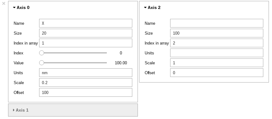
AxesManager ipywidgets GUI.
or the DataAxis, e.g:
>>> s.axes_manager["X"].gui()
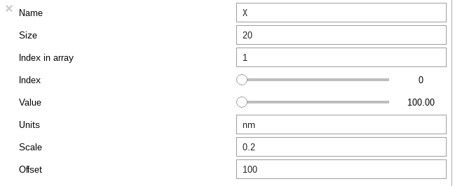
DataAxis ipywidgets GUI.
To simply change the “current position” (i.e. the indices of the navigation axes) you could use the navigation sliders:
>>> s.axes_manager.gui_navigation_sliders()
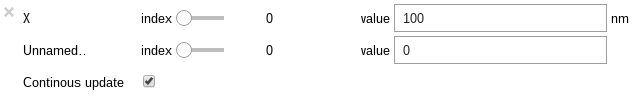
Navigation sliders ipywidgets GUI.
Alternatively, the “current position” can be changed programmatically by
directly accessing indices attribute of a Signal’s
AxesManager. This is particularly useful if trying to set
a specific location with which to initialize a model’s parameters to
sensible values before preforming a fit over an entire spectrum image. The
indices must be provided as a tuple, with the same length as the number of
navigation dimensions:
>>> s.axes_manager.indices = (5, 4)
Using quantity and converting units
The scale and the offset of each axis can be set and retrieved as quantity.
>>> s = hs.signals.Signal1D(np.arange(10))
>>> s.axes_manager[0].scale_as_quantity
1.0 dimensionless
>>> s.axes_manager[0].scale_as_quantity = '2.5 µm'
>>> s.axes_manager
<Axes manager, axes: (|10)>
            Name |   size |  index |  offset |   scale |  units
================ | ====== | ====== | ======= | ======= | ======
---------------- | ------ | ------ | ------- | ------- | ------
     <undefined> |     10 |        |       0 |     2.5 |     µm
>>> s.axes_manager[0].offset_as_quantity = '2.5 nm'
<Axes manager, axes: (|10)>
            Name |   size |  index |  offset |   scale |  units
================ | ====== | ====== | ======= | ======= | ======
---------------- | ------ | ------ | ------- | ------- | ------
     <undefined> |     10 |        |     2.5 | 2.5e+03 |     nm
Internally, HyperSpy uses the pint library to manage the scale and offset quantities. The scale_as_quantity and offset_as_quantity attributes return pint object:
>>> q = s.axes_manager[0].offset_as_quantity
>>> type(q) # q is a pint quantity object
pint.quantity.build_quantity_class.<locals>.Quantity
>>> q
2.5 nanometer
The convert_units method of the AxesManager converts units, which by default (no parameters provided) converts all axis units to an optimal units to avoid using too large or small number.
Each axis can also be converted individually using the convert_to_units method of the DataAxis:
>>> axis = hs.hyperspy.axes.DataAxis(size=10, scale=0.1, offset=10, units='mm')
>>> axis.scale_as_quantity
0.1 millimeter
>>> axis.convert_to_units('µm')
>>> axis.scale_as_quantity
100.0 micrometer
Saving Files
The data can be saved to several file formats. The format is specified by the extension of the filename.
>>> # load the data
>>> d = hs.load("example.tif")
>>> # save the data as a tiff
>>> d.save("example_processed.tif")
>>> # save the data as a png
>>> d.save("example_processed.png")
>>> # save the data as an hspy file
>>> d.save("example_processed.hspy")
Some file formats are much better at maintaining the information about how you processed your data. The preferred format in HyperSpy is hspy, which is based on the HDF5 format. This format keeps the most information possible.
There are optional flags that may be passed to the save function. See Saving data to files for more details.
Accessing and setting the metadata
When loading a file HyperSpy stores all metadata in the BaseSignal
original_metadata attribute. In addition,
some of those metadata and any new metadata generated by HyperSpy are stored in
metadata attribute.
>>> s = hs.load("NbO2_Nb_M_David_Bach,_Wilfried_Sigle_217.msa")
>>> s.metadata
├── original_filename = NbO2_Nb_M_David_Bach,_Wilfried_Sigle_217.msa
├── record_by = spectrum
├── signal_type = EELS
└── title = NbO2_Nb_M_David_Bach,_Wilfried_Sigle_217

>>> s.original_metadata
├── DATATYPE = XY
├── DATE =
├── FORMAT = EMSA/MAS Spectral Data File
├── NCOLUMNS = 1.0
├── NPOINTS = 1340.0
├── OFFSET = 120.0003
├── OWNER = eelsdatabase.net
├── SIGNALTYPE = ELS
├── TIME =
├── TITLE = NbO2_Nb_M_David_Bach,_Wilfried_Sigle_217
├── VERSION = 1.0
├── XPERCHAN = 0.5
├── XUNITS = eV
└── YUNITS =

>>> s.set_microscope_parameters(100, 10, 20)
>>> s.metadata
├── TEM
│   ├── EELS
│   │   └── collection_angle = 20
│   ├── beam_energy = 100
│   └── convergence_angle = 10
├── original_filename = NbO2_Nb_M_David_Bach,_Wilfried_Sigle_217.msa
├── record_by = spectrum
├── signal_type = EELS
└── title = NbO2_Nb_M_David_Bach,_Wilfried_Sigle_217

>>> s.metadata.TEM.microscope = "STEM VG"
>>> s.metadata
├── TEM
│   ├── EELS
│   │   └── collection_angle = 20
│   ├── beam_energy = 100
│   ├── convergence_angle = 10
│   └── microscope = STEM VG
├── original_filename = NbO2_Nb_M_David_Bach,_Wilfried_Sigle_217.msa
├── record_by = spectrum
├── signal_type = EELS
└── title = NbO2_Nb_M_David_Bach,_Wilfried_Sigle_217
Configuring HyperSpy
The behaviour of HyperSpy can be customised using the
Preferences class. The easiest way to do it is by
calling the gui() method:
>>> hs.preferences.gui()
This command should raise the Preferences user interface if one of the hyperspy gui packages are installed and enabled:
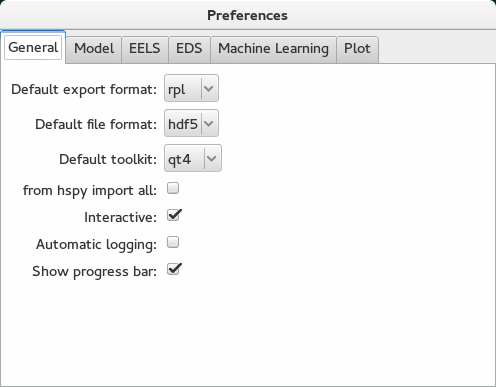
Preferences user interface.
New in version 1.3: Possibility to enable/disable GUIs in the
It is also possible to set the preferences programmatically. For example, to disable the traitsui GUI elements and save the changes to disk:
>>> hs.preferences.GUIs.enable_traitsui_gui = False
>>> hs.preferences.save()
Changed in version 1.3: The following items were removed from preferences:
General.default_export_format, General.lazy,
Model.default_fitter, Machine_learning.multiple_files,
Machine_learning.same_window, Plot.default_style_to_compare_spectra,
Plot.plot_on_load, Plot.pylab_inline, EELS.fine_structure_width,
EELS.fine_structure_active, EELS.fine_structure_smoothing,
EELS.synchronize_cl_with_ll, EELS.preedge_safe_window_width,
EELS.min_distance_between_edges_for_fine_structure.
Messages log
HyperSpy writes messages to the Python logger. The
default log level is “WARNING”, meaning that only warnings and more severe
event messages will be displayed. The default can be set in the
preferences. Alternatively, it can be set
using set_log_level() e.g.:
>>> import hyperspy.api as hs
>>> hs.set_log_level('INFO')
>>> hs.load(r'my_file.dm3')
INFO:hyperspy.io_plugins.digital_micrograph:DM version: 3
INFO:hyperspy.io_plugins.digital_micrograph:size 4796607 B
INFO:hyperspy.io_plugins.digital_micrograph:Is file Little endian? True
INFO:hyperspy.io_plugins.digital_micrograph:Total tags in root group: 15
<Signal2D, title: My file, dimensions: (|1024, 1024)