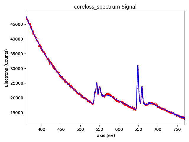
EELS curve fitting

Performs curve fitting to an EELS spectrum, plots the result and saves it as png file.

  0%|                                              | 0.00/42.3M [00:00<?, ?B/s]
  0%|                                      | 28.7k/42.3M [00:00<02:55, 240kB/s]
  0%|                                       | 110k/42.3M [00:00<01:47, 391kB/s]
  1%|▎                                     | 401k/42.3M [00:00<00:34, 1.21MB/s]
  2%|▉                                     | 974k/42.3M [00:00<00:15, 2.67MB/s]
  4%|█▌                                   | 1.72M/42.3M [00:00<00:09, 4.18MB/s]
  8%|███                                  | 3.49M/42.3M [00:00<00:04, 8.38MB/s]
 15%|█████▍                               | 6.16M/42.3M [00:00<00:02, 14.0MB/s]
 23%|████████▍                            | 9.62M/42.3M [00:00<00:01, 20.3MB/s]
 30%|███████████                          | 12.6M/42.3M [00:01<00:01, 23.3MB/s]
 39%|██████████████▎                      | 16.3M/42.3M [00:01<00:00, 27.5MB/s]
 46%|█████████████████                    | 19.4M/42.3M [00:01<00:00, 26.2MB/s]
 55%|████████████████████▎                | 23.2M/42.3M [00:01<00:00, 29.5MB/s]
 62%|██████████████████████▉              | 26.3M/42.3M [00:01<00:00, 29.7MB/s]
 70%|█████████████████████████▊           | 29.5M/42.3M [00:01<00:00, 30.6MB/s]
 77%|████████████████████████████▌        | 32.6M/42.3M [00:01<00:00, 30.6MB/s]
 86%|███████████████████████████████▊     | 36.4M/42.3M [00:01<00:00, 32.6MB/s]
 94%|██████████████████████████████████▋  | 39.6M/42.3M [00:01<00:00, 29.0MB/s]
  0%|                                              | 0.00/42.3M [00:00<?, ?B/s]
100%|██████████████████████████████████████| 42.3M/42.3M [00:00<00:00, 205GB/s]

  0%|                                              | 0.00/66.1M [00:00<?, ?B/s]
  0%|                                      | 14.3k/66.1M [00:00<08:27, 130kB/s]
  0%|                                      | 81.9k/66.1M [00:00<03:19, 330kB/s]
  0%|▏                                      | 232k/66.1M [00:00<01:28, 741kB/s]
  1%|▎                                     | 526k/66.1M [00:00<00:46, 1.42MB/s]
  2%|▊                                    | 1.43M/66.1M [00:00<00:16, 3.84MB/s]
  4%|█▌                                   | 2.85M/66.1M [00:00<00:08, 7.06MB/s]
  8%|███                                  | 5.39M/66.1M [00:00<00:04, 12.7MB/s]
 14%|█████▏                               | 9.21M/66.1M [00:00<00:02, 20.5MB/s]
 19%|███████                              | 12.7M/66.1M [00:00<00:02, 24.8MB/s]
 25%|█████████                            | 16.2M/66.1M [00:01<00:02, 24.1MB/s]
 30%|███████████▏                         | 19.9M/66.1M [00:01<00:01, 27.5MB/s]
 36%|█████████████▎                       | 23.7M/66.1M [00:01<00:01, 30.4MB/s]
 41%|███████████████▏                     | 27.2M/66.1M [00:01<00:01, 31.6MB/s]
 47%|█████████████████▎                   | 31.0M/66.1M [00:01<00:01, 33.3MB/s]
 52%|███████████████████▏                 | 34.4M/66.1M [00:01<00:00, 33.4MB/s]
 57%|█████████████████████▎               | 38.0M/66.1M [00:01<00:00, 34.2MB/s]
 63%|███████████████████████▎             | 41.6M/66.1M [00:01<00:00, 34.8MB/s]
 68%|█████████████████████████▏           | 45.1M/66.1M [00:01<00:00, 34.4MB/s]
 74%|███████████████████████████▎         | 48.7M/66.1M [00:02<00:00, 35.0MB/s]
 79%|█████████████████████████████▏       | 52.2M/66.1M [00:02<00:00, 34.8MB/s]
 85%|███████████████████████████████▎     | 55.9M/66.1M [00:02<00:00, 35.3MB/s]
 90%|█████████████████████████████████▎   | 59.6M/66.1M [00:02<00:00, 35.8MB/s]
 96%|███████████████████████████████████▍ | 63.2M/66.1M [00:02<00:00, 36.0MB/s]
  0%|                                              | 0.00/66.1M [00:00<?, ?B/s]
100%|██████████████████████████████████████| 66.1M/66.1M [00:00<00:00, 291GB/s]

import hyperspy.api as hs

s = hs.load("coreloss_spectrum.msa", signal_type="EELS")
low_loss = hs.load("lowloss_spectrum.msa", signal_type="EELS")

s.add_elements(("Mn", "O"))
s.set_microscope_parameters(
    beam_energy=300, convergence_angle=24.6, collection_angle=13.6
)

m = s.create_model(low_loss=low_loss)
m.enable_fine_structure()
m.multifit(kind="smart")
m.plot()

# one can also use the Dirac GOS by specifying the GOS parameter
m = s.create_model(low_loss=low_loss, GOS="dirac")
m.enable_fine_structure()
m.multifit(kind="smart")
m.plot()