Energy-Dispersive X-Rays Spectrometry (EDS)
The methods described here are specific to the following signals:
This chapter described step by step the analysis of an EDS spectrum (SEM or TEM).
Note
See also the EDS tutorials .
Spectrum loading and parameters
Data files used in the following examples can be downloaded using
>>> from urllib import urlretrieve
>>> url = 'http://cook.msm.cam.ac.uk//~hyperspy//EDS_tutorial//'
>>> urlretrieve(url + 'Ni_superalloy_1pix.msa', 'Ni_superalloy_1pix.msa')
>>> urlretrieve(url + 'Ni_superalloy_010.rpl', 'Ni_superalloy_010.rpl')
>>> urlretrieve(url + 'Ni_superalloy_010.raw', 'Ni_superalloy_010.raw')
Note
The sample and the data used in this chapter are described in P. Burdet, et al., Acta Materialia, 61, p. 3090-3098 (2013) (see abstract).
Loading
All data are loaded with the load() function, as described in details in
Loading files. HyperSpy is able to import different formats,
among them ”.msa” and ”.rpl” (the raw format of Oxford Instrument and Brucker).
Here is three example for files exported by Oxford Instrument software (INCA). For a single spectrum:
>>> s = hs.load("Ni_superalloy_1pix.msa")
>>> s
<Signal1D, title: Signal1D, dimensions: (|1024)>
For a spectrum image (The .rpl file is recorded as an image in this example,
The method as_signal1D() set it back to a one
dimensional signal with the energy axis in first position):
>>> si = hs.load("Ni_superalloy_010.rpl").as_spectrum(0)
>>> si
<Signal1D, title: , dimensions: (256, 224|1024)>
For a stack of spectrum images (The “*” replace all chains of string, in this example 01, 02, 03,...):
>>> si4D = hs.load("Ni_superalloy_0*.rpl", stack=True)
>>> si4D = si4D.as_signal1D(0)
>>> si4D
<Signal1D, title:, dimensions: (256, 224, 2|1024)>
Microscope and detector parameters
First, the type of microscope (“EDS_TEM” or “EDS_SEM”) needs to be set with the
set_signal_type() method. The class of the
object is thus assigned, and specific EDS methods become available.
>>> s = hs.load("Ni_superalloy_1pix.msa")
>>> s.set_signal_type("EDS_SEM")
>>> s
<EDSSEMSpectrum, title: Spectrum, dimensions: (|1024)>
or as an argument of the load() function:
>>> s = hs.load("Ni_superalloy_1pix.msa", signal_type="EDS_SEM")
>>> s
<EDSSEMSpectrum, title: Spectrum, dimensions: (|1024)>
The main values for the microscope parameters are
automatically imported from the file, if existing. The microscope and
detector parameters are stored in stored in the
metadata
attribute (see Metadata structure). These parameters can be displayed
as follow:
>>> s = hs.load("Ni_superalloy_1pix.msa", signal_type="EDS_SEM")
>>> s.metadata.Acquisition_instrument.SEM
├── Detector
│   └── EDS
│       ├── azimuth_angle = 63.0
│       ├── elevation_angle = 35.0
│       ├── energy_resolution_MnKa = 130.0
│       ├── live_time = 0.006855
│       └── real_time = 0.0
├── beam_current = 0.0
├── beam_energy = 15.0
└── tilt_stage = 38.0
These parameters can be set directly:
>>> s = hs.load("Ni_superalloy_1pix.msa", signal_type="EDS_SEM")
>>> s.metadata.Acquisition_instrument.SEM.beam_energy = 30
or with the
set_microscope_parameters() method:
>>> s = hs.load("Ni_superalloy_1pix.msa", signal_type="EDS_SEM")
>>> s.set_microscope_parameters(beam_energy = 30)
or raising the gui:
>>> s = hs.load("Ni_superalloy_1pix.msa", signal_type="EDS_SEM")
>>> s.set_microscope_parameters()
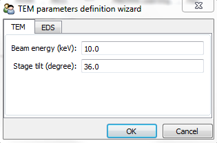
EDS microscope parameters preferences window.
If the microscope and detector parameters are not written in the original file, some
of them are set by default. The default values can be changed in the
Preferences class (see preferences).
>>> hs.preferences.EDS.eds_detector_elevation = 37
or raising the gui:
>>> hs.preferences.gui()

EDS preferences window.
Energy axis
The main values for the energy axis are automatically imported from the file, if existing. The properties of the energy axis can be set manually with the AxesManager.
(see Axis properties for more info):
>>> si = hs.load("Ni_superalloy_010.rpl", signal_type="EDS_TEM").as_spectrum(0)
>>> si.axes_manager[-1].name = 'E'
>>> si.axes_manager['E'].units = 'keV'
>>> si.axes_manager['E'].scale = 0.01
>>> si.axes_manager['E'].offset = -0.1
or with the gui() method:
>>> si.axes_manager.gui()
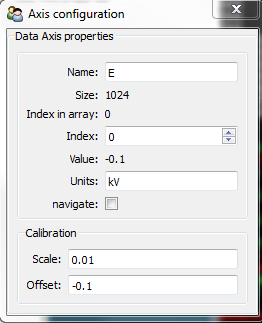
Axis properties window.
Describing the sample
The description of the sample is stored in metadata.Sample (in the
metadata attribute). It can be displayed as
follow:
>>> s = hs.datasets.example_signals.EDS_TEM_Spectrum()
>>> s.add_lines()
>>> s.metadata.Sample.thickness = 100
>>> s.metadata.Sample
├── description = FePt bimetallic nanoparticles
├── elements = ['Fe', 'Pt']
├── thickness = 100
└── xray_lines = ['Fe_Ka', 'Pt_La']
The following methods are either called “set” or “add”. When “set” methods erases all previously defined values, the “add” methods add the values to the previously defined values.
Elements
The elements present in the sample can be defined with the
set_elements() and
add_elements() methods. Only element
abbreviations are accepted:
>>> s = hs.datasets.example_signals.EDS_TEM_Spectrum()
>>> s.set_elements(['Fe', 'Pt'])
>>> s.add_elements(['Cu'])
>>> s.metadata.Sample
└── elements = ['Cu', 'Fe', 'Pt']
X-ray lines
Similarly, the X-ray lines can be defined with the
set_lines() and
add_lines() methods. The corresponding
elements will be added automatically. Several lines per elements can be defined.
>>> s = hs.datasets.example_signals.EDS_TEM_Spectrum()
>>> s.set_elements(['Fe', 'Pt'])
>>> s.set_lines(['Fe_Ka', 'Pt_La'])
>>> s.add_lines(['Fe_La'])
>>> s.metadata.Sample
├── elements = ['Fe', 'Pt']
└── xray_lines = ['Fe_Ka', 'Fe_La', 'Pt_La']
These methods can be used automatically, if the beam energy is set. The most excited X-ray line is selected per element (highest energy above an overvoltage of 2 (< beam energy / 2)).
>>> s = hs.datasets.example_signals.EDS_SEM_Spectrum()
>>> s.set_elements(['Al', 'Cu', 'Mn'])
>>> s.set_microscope_parameters(beam_energy=30)
>>> s.add_lines()
>>> s.metadata.Sample
├── elements = ['Al', 'Cu', 'Mn']
└── xray_lines = ['Al_Ka', 'Cu_Ka', 'Mn_Ka']
>>> s.set_microscope_parameters(beam_energy=10)
>>> s.set_lines([])
>>> s.metadata.Sample
├── elements = ['Al', 'Cu', 'Mn']
└── xray_lines = ['Al_Ka', 'Cu_La', 'Mn_La']
A warning is raised, if setting a X-ray lines higher than the beam energy.
>>> s = hs.datasets.example_signals.EDS_SEM_Spectrum()
>>> s.set_elements(['Mn'])
>>> s.set_microscope_parameters(beam_energy=5)
>>> s.add_lines(['Mn_Ka'])
Warning: Mn Ka is above the data energy range.
Element database
An elemental database is available with the energy of the X-ray lines.
>>> hs.material.elements.Fe.General_properties
├── Z = 26
├── atomic_weight = 55.845
└── name = iron
>>> hs.material.elements.Fe.Physical_properties
└── density (g/cm^3) = 7.874
>>> hs.material.elements.Fe.Atomic_properties.Xray_lines
├── Ka
│   ├── energy (keV) = 6.404
│   └── weight = 1.0
├── Kb
│   ├── energy (keV) = 7.0568
│   └── weight = 0.1272
├── La
│   ├── energy (keV) = 0.705
│   └── weight = 1.0
├── Lb3
│   ├── energy (keV) = 0.792
│   └── weight = 0.02448
├── Ll
│   ├── energy (keV) = 0.615
│   └── weight = 0.3086
└── Ln
    ├── energy (keV) = 0.62799
    └── weight = 0.12525
Plotting
As decribed in visualisation, the
plot() method can be used:
>>> s = hs.datasets.example_signals.EDS_SEM_Spectrum()
>>> s.plot()
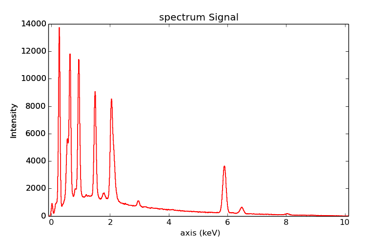
EDS spectrum.
An example of plotting EDS data of higher dimension (3D SEM-EDS) is given in visualisation multi-dimension.
Plot X-ray lines
New in version 0.8.
X-ray lines can be labbeled on a plot with
plot(). The lines are
either given, either retrieved from “metadata.Sample.Xray_lines”,
or selected with the same method as
add_lines() using the
elements in “metadata.Sample.elements”.
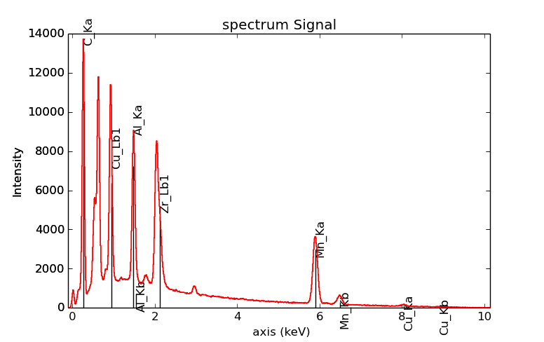
>>> s = hs.datasets.example_signals.EDS_SEM_Spectrum()
>>> s.add_elements(['C','Mn','Cu','Al','Zr'])
>>> s.plot(True)
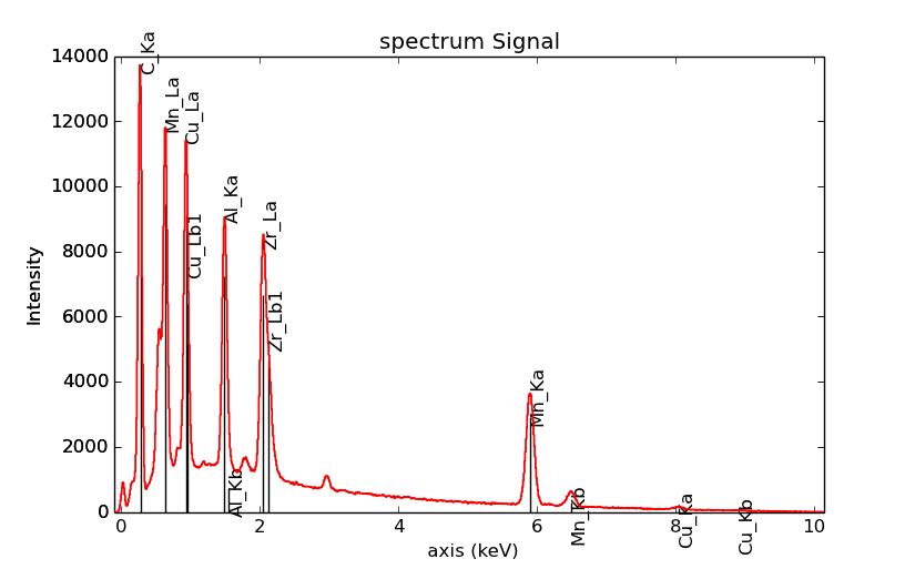
EDS spectrum plot with line markers.
Selecting certain type of lines:
>>> s = hs.datasets.example_signals.EDS_SEM_Spectrum()
>>> s.add_elements(['C','Mn','Cu','Al','Zr'])
>>> s.plot(True, only_lines=['Ka','b'])
EDS spectrum plot with a selection of line markers.
Get lines intensity
Data files used in the following examples can be downloaded using
>>> from urllib import urlretrieve
>>> url = 'http://cook.msm.cam.ac.uk//~hyperspy//EDS_tutorial//'
>>> urlretrieve(url + 'core_shell.hdf5', 'core_shell.hdf5')
Note
The sample and the data used in this section are described in D. Roussow et al., Nano Lett, 10.1021/acs.nanolett.5b00449 (2015).
New in version 0.8.
The width of integration is defined by extending the energy resolution of Mn Ka to the peak energy (“energy_resolution_MnKa” in metadata).
>>> s = hs.load('core_shell.hdf5')
>>> s.get_lines_intensity(['Fe_Ka'], plot_result=True)
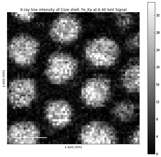
Iron map as computed and displayed by get_lines_intensity.
The X-ray lines defined in “metadata.Sample.Xray_lines” (see above) are used by default.
>>> s = hs.load('core_shell.hdf5')
>>> s.set_lines(['Fe_Ka', 'Pt_La'])
>>> s.get_lines_intensity()
[<Signal2D, title: X-ray line intensity of Core shell: Fe_Ka at 6.40 keV, dimensions: (|64, 64)>,
<Signal2D, title: X-ray line intensity of Core shell: Pt_La at 9.44 keV, dimensions: (|64, 64)>]
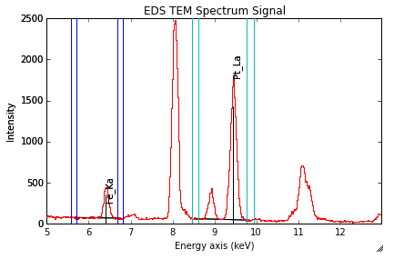
The windows of integration can be visualised using plot() method
>>> s = hs.datasets.example_signals.EDS_TEM_Spectrum()[5.:13.]
>>> s.add_lines()
>>> s.plot(integration_windows='auto')
EDS spectrum with integration windows markers.
Background subtraction
New in version 0.8.
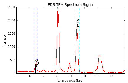
The background can be subtracted from the X-ray intensities with the get_lines_intensity() method. The background value is obtained by averaging the intensity in two windows on each side of the X-ray line. The position of the windows can be estimated with the estimate_background_windows() method and can be plotted with the plot() method as follow. The integration windows are plotted with dashed lines.
>>> s = hs.datasets.example_signals.EDS_TEM_Spectrum()[5.:13.]
>>> s.add_lines()
>>> bw = s.estimate_background_windows(line_width=[5.0, 2.0])
>>> s.plot(background_windows=bw)
>>> s.get_lines_intensity(background_windows=bw, plot_result=True)
EDS spectrum with background subtraction markers.
Quantification
New in version 0.8.
One TEM quantification method (Cliff-Lorimer) is implemented so far.
Quantification can be applied from the intensities (background subtracted) with the quantification() method. The required k-factors can be usually found in the EDS manufacturer software.
>>> s = hs.datasets.example_signals.EDS_TEM_Spectrum()
>>> s.add_lines()
>>> kfactors = [1.450226, 5.075602] #For Fe Ka and Pt La
>>> bw = s.estimate_background_windows(line_width=[5.0, 2.0])
>>> intensities = s.get_lines_intensity(background_windows=bw)
>>> weight_percent = s.quantification(intensities, kfactors, plot_result=True)
Fe (Fe_Ka): Composition = 4.96 weight percent
Pt (Pt_La): Composition = 95.04 weight percent
The obtained composition is in weight percent. It can be changed transformed into atomic percent either with the option quantification():
>>> # With s, intensities and kfactors from before
>>> s.quantification(intensities, kfactors, plot_result=True,
>>>                  composition_units='atomic')
Fe (Fe_Ka): Composition = 15.41 atomic percent
Pt (Pt_La): Composition = 84.59 atomic percent
either with weight_to_atomic(). The reverse method is atomic_to_weight().
>>> # With weight_percent from before
>>> atomic_percent = hs.material.weight_to_atomic(weight_percent)