Getting started
Starting HyperSpy
HyperSpy is a Python library for multi-dimensional data analysis. HyperSpy’s API can be imported as any other Python library as follows:
>>> import hyperspy.api as hs
The most common way of using HyperSpy is interactively using interactive
computing package IPython. In all operating systems (OS)
you can start IPython by opening a system terminal and executing ipython,
optionally followed by the frontend. In most cases, the most agreeable way
to work with HyperSpy interactively is using the Jupyter Notebook (previously known as the IPython Notebook), which can be
started as follows:
$ jupyter notebook
Some may find it more convenient to start Jupyter/IPython from the file manager context menu or by double-clicking a notebook file.
Typically you will need to set up IPython for interactive plotting with
matplotlib using the
%matplotlib magic before executing any plotting command. So, typically,
after starting IPython, you can import
HyperSpy and set up interactive matplotlib plotting by executing the following
two lines in the IPython terminal:
In [1]: %matplotlib qt
In [2]: import hyperspy.api as hs
We also fully support the wx backend. Other backends are supported for plotting but some features such as navigation sliders may be missing.
Warning
When using the qt4 backend in Python 2 the matplotlib magic must be executed after importing hyperspy and qt must be the default hyperspy backend.
Note
When running in a headless system it is necessary to set the matplotlib backend appropiately to avoid a cannot connect to X server error, for example as follows:
In [1]: import matplotlib
In [2]: matplotlib.rcParams["backend"] = "Agg"
In [3]: import hyperspy.api as hs
This documentation assumes that numpy and matplotlib are also imported as follows:
>>> import numpy as np
>>> import matplotlib.pyplot as plt
Warning
Starting HyperSpy using the hyperspy starting script and the
%hyperspy IPython magic is now deprecated and will be removed in
Hyperspy 1.0. The IPython magic does not work with IPython 4 and
above.
Getting help
When using IPython, the documentation (docstring in Python jargon) can be accessed by adding a question mark to the name of a function. e.g.:
>>> hs?
>>> hs.load?
>>> hs.signals?
This syntax is a shortcut to the standard way one of displaying the help associated to a given functions (docstring in Python jargon) and it is one of the many features of IPython, which is the interactive python shell that HyperSpy uses under the hood.
Please note that the documentation of the code is a work in progress, so not all the objects are documented yet.
Up-to-date documentation is always available in the HyperSpy website.
Autocompletion
Another useful IPython feature is the autocompletion of commands and filenames using the tab and arrow keys. It is highly recommended to read the Ipython documentation (specially their Getting started section) for many more useful features that will boost your efficiency when working with HyperSpy/Python interactively.
Loading data
Once hyperspy is running, to load from a supported file format (see Supported formats) simply type:
>>> s = hs.load("filename")
Hint
The load function returns an object that contains data read from the file.
We assign this object to the variable s but you can choose any (valid)
variable name you like. for the filename, don’t forget to include the
quotation marks and the file extension.
If no argument is passed to the load function, a window will be raised that allows to select a single file through your OS file manager, e.g.:
>>> # This raises the load user interface
>>> s = hs.load()
It is also possible to load multiple files at once or even stack multiple files. For more details read Loading files: the load function
“Loading” data from a numpy array
HyperSpy can operate on any numpy array by assigning it to a Signal class.
This is useful e.g. for loading data stored in a format that is not yet
supported by HyperSpy—supposing that they can be read with another Python
library—or to explore numpy arrays generated by other Python
libraries. Simply select the most appropiate signal from the
signals module and create a new instance by passing a numpy array
to the constructor e.g.
>>> my_np_array = np.random.random((10,20,100))
>>> s = hs.signals.Signal1D(my_np_array)
>>> s
<Signal1D, title: , dimensions: (20, 10|100)>
The numpy array is stored in the data attribute
of the signal class.
Setting axis properties
The axes are managed and stored by the AxesManager class
that is stored in the axes_manager attribute of
the signal class. The indidual axes can be accessed by indexing the AxesManager
e.g.
>>> s = hs.signals.Signal1D(np.random.random((10, 20 , 100)))
>>> s
<Signal1D, title: , dimensions: (20, 10|100)>
>>> s.axes_manager
<Axes manager, axes: (<Unnamed 0th axis, size: 20, index: 0>, <Unnamed 1st
axis, size: 10, index: 0>|<Unnamed 2nd axis, size: 100>)>
>>> s.axes_manager[0]
<Unnamed 0th axis, size: 20, index: 0>
The axis properties can be set by setting the DataAxis
attributes e.g.
>>> s.axes_manager[0].name = "X"
>>> s.axes_manager[0]
<X axis, size: 20, index: 0>
Once the name of an axis has been defined it is possible to request it by its name e.g.:
>>> s.axes_manager["X"]
<X axis, size: 20, index: 0>
>>> s.axes_manager["X"].scale = 0.2
>>> s.axes_manager["X"].units = nm
>>> s.axes_manager["X"].offset = 100
It is also possible to set the axes properties using a GUI by calling the
gui() method of the AxesManager.
Saving Files
The data can be saved to several file formats. The format is specified by the extension of the filename.
>>> # load the data
>>> d = hs.load("example.tif")
>>> # save the data as a tiff
>>> d.save("example_processed.tif")
>>> # save the data as a png
>>> d.save("example_processed.png")
>>> # save the data as an hdf5 file
>>> d.save("example_processed.hdf5")
Some file formats are much better at maintaining the information about how you processed your data. The preferred format in HyperSpy is hdf5, the hierarchical data format. This format keeps the most information possible.
There are optional flags that may be passed to the save function. See Saving data to files for more details.
Accessing and setting the metadata
When loading a file HyperSpy stores all metadata in the Signal
original_metadata attribute. In addition, some of
those metadata and any new metadata generated by HyperSpy are stored in
metadata attribute.
>>> s = hs.load("NbO2_Nb_M_David_Bach,_Wilfried_Sigle_217.msa")
>>> s.metadata
├── original_filename = NbO2_Nb_M_David_Bach,_Wilfried_Sigle_217.msa
├── record_by = spectrum
├── signal_origin =
├── signal_type = EELS
└── title = NbO2_Nb_M_David_Bach,_Wilfried_Sigle_217

>>> s.original_metadata
├── DATATYPE = XY
├── DATE =
├── FORMAT = EMSA/MAS Spectral Data File
├── NCOLUMNS = 1.0
├── NPOINTS = 1340.0
├── OFFSET = 120.0003
├── OWNER = eelsdatabase.net
├── SIGNALTYPE = ELS
├── TIME =
├── TITLE = NbO2_Nb_M_David_Bach,_Wilfried_Sigle_217
├── VERSION = 1.0
├── XPERCHAN = 0.5
├── XUNITS = eV
└── YUNITS =

>>> s.set_microscope_parameters(100, 10, 20)
>>> s.metadata
├── TEM
│   ├── EELS
│   │   └── collection_angle = 20
│   ├── beam_energy = 100
│   └── convergence_angle = 10
├── original_filename = NbO2_Nb_M_David_Bach,_Wilfried_Sigle_217.msa
├── record_by = spectrum
├── signal_origin =
├── signal_type = EELS
└── title = NbO2_Nb_M_David_Bach,_Wilfried_Sigle_217

>>> s.metadata.TEM.microscope = "STEM VG"
>>> s.metadata
├── TEM
│   ├── EELS
│   │   └── collection_angle = 20
│   ├── beam_energy = 100
│   ├── convergence_angle = 10
│   └── microscope = STEM VG
├── original_filename = NbO2_Nb_M_David_Bach,_Wilfried_Sigle_217.msa
├── record_by = spectrum
├── signal_origin =
├── signal_type = EELS
└── title = NbO2_Nb_M_David_Bach,_Wilfried_Sigle_217
Configuring HyperSpy
The behaviour of HyperSpy can be customised using the
Preferences class. The easiest way to do it is by
calling the gui() method:
>>> hs.preferences.gui()
This command should raise the Preferences user interface:
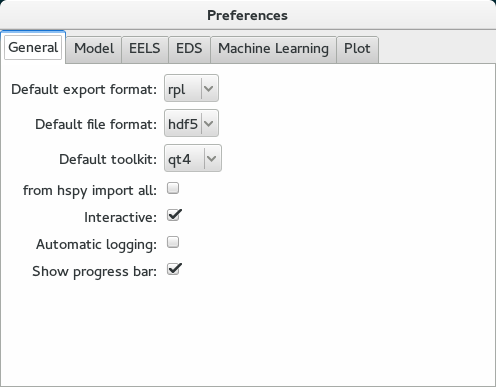
Preferences user interface.