Energy-Dispersive X-ray Spectrometry (EDS)¶

Signal1D loading and parameters¶

The sample and data used in this section are described in [Burdet2013], and can be downloaded using:

>>> from urllib import urlretrieve
>>> url = 'http://cook.msm.cam.ac.uk//~hyperspy//EDS_tutorial//'
>>> urlretrieve(url + 'Ni_superalloy_1pix.msa', 'Ni_superalloy_1pix.msa')
>>> urlretrieve(url + 'Ni_superalloy_010.rpl', 'Ni_superalloy_010.rpl')
>>> urlretrieve(url + 'Ni_superalloy_010.raw', 'Ni_superalloy_010.raw')

>>> s = hs.load("Ni_superalloy_1pix.msa")
>>> s
<Signal1D, title: Signal1D, dimensions: (|1024)>

>>> si = hs.load("Ni_superalloy_010.rpl").as_signal1D(0)
>>> si
<Signal1D, title: , dimensions: (256, 224|1024)>

>>> si4D = hs.load("Ni_superalloy_0*.rpl", stack=True)
>>> si4D = si4D.as_signal1D(0)
>>> si4D
<Signal1D, title:, dimensions: (256, 224, 2|1024)>

Microscope and detector parameters¶

First, the signal type (“EDS_TEM” or “EDS_SEM”) needs to be set with the set_signal_type() method. By assigning the class of the object, specific EDS methods are made available.

>>> s = hs.load("Ni_superalloy_1pix.msa")
>>> s.set_signal_type("EDS_SEM")
>>> s
<EDSSEMSpectrum, title: Signal1D, dimensions: (|1024)>

You can also specify the signal type as an argument of the load() function:

>>> s = hs.load("Ni_superalloy_1pix.msa", signal_type="EDS_SEM")
>>> s
<EDSSEMSpectrum, title: Signal1D, dimensions: (|1024)>

HyperSpy will automatically load any existing microscope parameters from the file, and store them in the metadata attribute (see Metadata structure). These parameters can be displayed as follows:

>>> s = hs.load("Ni_superalloy_1pix.msa", signal_type="EDS_SEM")
>>> s.metadata.Acquisition_instrument.SEM
├── Detector
│   └── EDS
│       ├── azimuth_angle = 63.0
│       ├── elevation_angle = 35.0
│       ├── energy_resolution_MnKa = 130.0
│       ├── live_time = 0.006855
│       └── real_time = 0.0
├── beam_current = 0.0
├── beam_energy = 15.0
└── tilt_stage = 38.0

You can also set these parameters directly:

>>> s = hs.load("Ni_superalloy_1pix.msa", signal_type="EDS_SEM")
>>> s.metadata.Acquisition_instrument.SEM.beam_energy = 30

or by using the set_microscope_parameters() method:

>>> s = hs.load("Ni_superalloy_1pix.msa", signal_type="EDS_SEM")
>>> s.set_microscope_parameters(beam_energy = 30)

or through the GUI:

>>> s = hs.load("Ni_superalloy_1pix.msa", signal_type="EDS_SEM")
>>> s.set_microscope_parameters()

EDS microscope parameters preferences window

Any microscope and detector parameters that are not found in the imported file will be set by default. These default values can be changed in the Preferences class (see preferences).

>>> hs.preferences.EDS.eds_detector_elevation = 37

or through the GUI:

>>> hs.preferences.gui()

EDS preferences window

Energy axis¶

The size, scale and units of the energy axis are automatically imported from the imported file, where they exist. These properties can also be set or adjusted manually with the AxesManager (see Axis properties for more info):

>>> si = hs.load("Ni_superalloy_010.rpl", signal_type="EDS_TEM").as_signal1D(0)
>>> si.axes_manager[-1].name = 'E'
>>> si.axes_manager['E'].units = 'keV'
>>> si.axes_manager['E'].scale = 0.01
>>> si.axes_manager['E'].offset = -0.1

or through the GUI:

>>> si.axes_manager.gui()

Axis properties window

>>> # s1pixel contains all the parameters
>>> s1pixel = hs.load("Ni_superalloy_1pix.msa", signal_type="EDS_TEM")
>>>
>>> # si contains no parameters
>>> si = hs.load("Ni_superalloy_010.rpl", signal_type="EDS_TEM").as_signal1D(0)
>>>
>>> # Copy all the properties of s1pixel to si
>>> si.get_calibration_from(s1pixel)

Describing the sample¶

The description of the sample is also stored in the metadata attribute. It can be displayed using:

>>> s = hs.datasets.example_signals.EDS_TEM_Spectrum()
>>> s.add_lines()
>>> s.metadata.Sample.thickness = 100
>>> s.metadata.Sample
├── description = FePt bimetallic nanoparticles
├── elements = ['Fe', 'Pt']
├── thickness = 100
└── xray_lines = ['Fe_Ka', 'Pt_La']

The following methods are either called “set” or “add”.

• “set” methods overwrite previously defined values
• “add” methods add to the previously defined values

>>> s = hs.datasets.example_signals.EDS_TEM_Spectrum()
>>> s.set_elements(['Fe', 'Pt'])
>>> s.add_elements(['Cu'])
>>> s.metadata.Sample
└── elements = ['Cu', 'Fe', 'Pt']

>>> s = hs.datasets.example_signals.EDS_TEM_Spectrum()
>>> s.set_elements(['Fe', 'Pt'])
>>> s.set_lines(['Fe_Ka', 'Pt_La'])
>>> s.add_lines(['Fe_La'])
>>> s.metadata.Sample
├── elements = ['Fe', 'Pt']
└── xray_lines = ['Fe_Ka', 'Fe_La', 'Pt_La']

>>> s = hs.datasets.example_signals.EDS_SEM_Spectrum()
>>> s.set_elements(['Al', 'Cu', 'Mn'])
>>> s.set_microscope_parameters(beam_energy=30)
>>> s.add_lines()
>>> s.metadata.Sample
├── elements = ['Al', 'Cu', 'Mn']
└── xray_lines = ['Al_Ka', 'Cu_Ka', 'Mn_Ka']

>>> s.set_microscope_parameters(beam_energy=10)
>>> s.set_lines([])
>>> s.metadata.Sample
├── elements = ['Al', 'Cu', 'Mn']
└── xray_lines = ['Al_Ka', 'Cu_La', 'Mn_La']

>>> s = hs.datasets.example_signals.EDS_SEM_Spectrum()
>>> s.set_elements(['Mn'])
>>> s.set_microscope_parameters(beam_energy=5)
>>> s.add_lines(['Mn_Ka'])
Warning: Mn Ka is above the data energy range.

>>> hs.material.elements.Fe.General_properties
├── Z = 26
├── atomic_weight = 55.845
└── name = iron
>>> hs.material.elements.Fe.Physical_properties
└── density (g/cm^3) = 7.874
>>> hs.material.elements.Fe.Atomic_properties.Xray_lines
├── Ka
│   ├── energy (keV) = 6.404
│   └── weight = 1.0
├── Kb
│   ├── energy (keV) = 7.0568
│   └── weight = 0.1272
├── La
│   ├── energy (keV) = 0.705
│   └── weight = 1.0
├── Lb3
│   ├── energy (keV) = 0.792
│   └── weight = 0.02448
├── Ll
│   ├── energy (keV) = 0.615
│   └── weight = 0.3086
└── Ln
    ├── energy (keV) = 0.62799
    └── weight = 0.12525

>>> s = hs.datasets.example_signals.EDS_SEM_Spectrum()
>>> P = s.find_peaks1D_ohaver(maxpeakn=1)[0]
>>> hs.eds.get_xray_lines_near_energy(P['position'], only_lines=['a', 'b'])
['C_Ka', 'Ca_La', 'B_Ka']

>>> hs.material.mass_absorption_coefficient(
>>>     element='Al', energies=['C_Ka','Al_Ka'])
array([ 26330.38933818,    372.02616732])

>>> hs.material.mass_absorption_mixture(
>>>     elements=['Al','Zn'], weight_percent=[50,50], energies='Al_Ka')
2587.4161643905127

Plotting¶

You can visualize an EDS spectrum using the plot() method (see visualisation). For example:

>>> s = hs.datasets.example_signals.EDS_SEM_Spectrum()
>>> s.plot()

EDS spectrum

An example of multi-dimensional EDS data (e.g. 3D SEM-EDS) is given in visualisation multi-dimension.

Plotting X-ray lines¶

New in version 0.8.

X-ray lines can be added as plot labels with plot(). The lines are either retrieved from “metadata.Sample.Xray_lines”, or selected with the same method as add_lines() using the elements in “metadata.Sample.elements”.

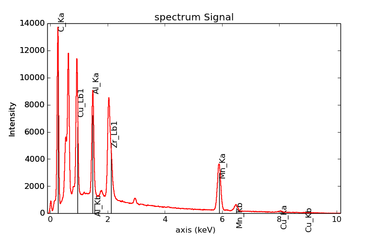
>>> s = hs.datasets.example_signals.EDS_SEM_Spectrum()
>>> s.add_elements(['C','Mn','Cu','Al','Zr'])
>>> s.plot(True)

EDS spectrum plot with line markers

You can also select a subset of lines to label:

>>> s = hs.datasets.example_signals.EDS_SEM_Spectrum()
>>> s.add_elements(['C','Mn','Cu','Al','Zr'])
>>> s.plot(True, only_lines=['Ka','b'])

EDS spectrum plot with a selection of line markers

Geting the intensity of an X-ray line¶

The sample and data used in this section are described in [Rossouw2015], and can be downloaded using:

>>> from urllib import urlretrieve
>>> url = 'http://cook.msm.cam.ac.uk//~hyperspy//EDS_tutorial//'
>>> urlretrieve(url + 'core_shell.hdf5', 'core_shell.hdf5')

The width of integration is defined by extending the energy resolution of Mn Ka to the peak energy (“energy_resolution_MnKa” in metadata):

>>> s = hs.load('core_shell.hdf5')
>>> s.get_lines_intensity(['Fe_Ka'], plot_result=True)

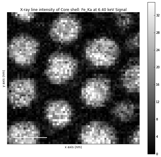
Iron map as computed and displayed by get_lines_intensity

The X-ray lines defined in “metadata.Sample.Xray_lines” (see above) are used by default:

>>> s = hs.load('core_shell.hdf5')
>>> s.set_lines(['Fe_Ka', 'Pt_La'])
>>> s.get_lines_intensity()
[<Signal2D, title: X-ray line intensity of Core shell: Fe_Ka at 6.40 keV, dimensions: (|64, 64)>,
<Signal2D, title: X-ray line intensity of Core shell: Pt_La at 9.44 keV, dimensions: (|64, 64)>]

Finally, the windows of integration can be visualised using plot() method:

>>> s = hs.datasets.example_signals.EDS_TEM_Spectrum()[5.:13.]
>>> s.add_lines()
>>> s.plot(integration_windows='auto')

EDS spectrum with integration windows markers

Background subtraction¶

New in version 0.8.

The background can be subtracted from the X-ray intensities with get_lines_intensity(). The background value is obtained by averaging the intensity in two windows on each side of the X-ray line. The position of the windows can be estimated using estimate_background_windows(), and can be plotted using plot():

>>> s = hs.datasets.example_signals.EDS_TEM_Spectrum()[5.:13.]
>>> s.add_lines()
>>> bw = s.estimate_background_windows(line_width=[5.0, 2.0])
>>> s.plot(background_windows=bw)
>>> s.get_lines_intensity(background_windows=bw, plot_result=True)

EDS spectrum with background subtraction markers.

EDS Quantification¶

HyperSpy now includes three methods for EDS quantification:

• Cliff-Lorimer
• Zeta-factors
• Ionization cross sections

Quantification must be applied to the background-subtracted intensities, which can be found using get_lines_intensity(). The quantification of these intensities can then be calculated using quantification().

The quantification method needs be specified as either ‘CL’, ‘zeta’, or ‘cross_section’. If no method is specified, the function will raise an exception.

A list of factors or cross sections should be supplied in the same order as the listed intensities (please note that HyperSpy intensities in :py:meth:~._signals.eds.EDSSpectrum.get_lines_intensity are in alphabetical order).

A set of k-factors can be usually found in the EDS manufacturer software although determination from standard samples for the particular instrument used is usually preferable. In the case of zeta-factors and cross sections, these must be determined experimentally using standards.

Zeta-factors should be provided in units of kg/m^2. The method is described further in [Watanabe1996] and [Watanabe2006] . Cross sections should be provided in units of barns (b). Further details on the cross section method can be found in [MacArthur2016] . Conversion between zeta-factors and cross sections is possible using :py:meth:~._misc.eds.util.edx_cross_section_to_zeta or :py:meth:~._misc.eds.util.zeta_to_edx_cross_section .

Using the Cliff-Lorimer method as an example, quantification can be carried out as follows:

>>> s = hs.datasets.example_signals.EDS_TEM_Spectrum()
>>> s.add_lines()
>>> kfactors = [1.450226, 5.075602] #For Fe Ka and Pt La
>>> bw = s.estimate_background_windows(line_width=[5.0, 2.0])
>>> intensities = s.get_lines_intensity(background_windows=bw)
>>> atomic_percent = s.quantification(intensities, method='CL', kfactors)
Fe (Fe_Ka): Composition = 15.41 atomic percent
Pt (Pt_La): Composition = 84.59 atomic percent

The obtained composition is in atomic percent, by default. However, it can be transformed into weight percent either with the option quantification():

>>> # With s, intensities and kfactors from before
>>> s.quantification(intensities, method='CL',kfactors,
>>>                  composition_units='weight')
Fe (Fe_Ka): Composition = 4.96 weight percent
Pt (Pt_La): Composition = 95.04 weight percent

or using atomic_to_weight():

>>> # With atomic_percent from before
>>> weight_percent = hs.material.atomic_to_weight(atomic_percent)

The reverse method is weight_to_atomic().

The zeta-factor method needs both the ‘beam_current’ (in nA) and the acquisition or dwell time (referred to as ‘real_time’ in seconds) in order to obtain an accurate quantification. Both of the these parameters can be assigned to the metadata using:

>>> s.set_microscope_parameters(beam_current=0.5)
>>> s.set_microscope_parameters(real_time=1.5)

If these parameters are not set, the code will produce an error. The zeta-factor method will produce two sets of results. Index [0] contains the composition maps for each element in atomic percent, and index [1] contains the mass-thickness map.

The cross section method needs the ‘beam_current’, dwell time (‘real_time’) and probe area in order to obtain an accurate quantification. The ‘beam_current’ and ‘real_time’ can be set as shown above. The ‘probe_area’ (in nm^2) can be defined in two different ways.

If the probe diameter is narrower than the pixel width, then the probe is being under-sampled and an estimation of the probe area needs to be used. This can be added to the metadata with:

Alternatively, if sub-pixel scanning is used (or the spectrum map was recorded at a high spatial sampling and subsequently binned into much larger pixels) then the illumination area becomes the pixel area of the spectrum image. This is a much more accurate approach for quantitative EDS and should be used where possible. The pixel width could either be added to the metadata by putting the pixel area in as the ‘probe_area’ (above) or by calibrating the spectrum image (see Setting axis properties).

Either approach will provide an illumination area for the cross_section quantification. If the pixel width is not set, the code will still run with the default value of 1 nm with a warning message to remind the user that this is the case.

The cross section method will produce two sets of results. Index [0] contains the composition maps for each element in atomic percent and index [1] is the number of atoms per pixel for each element.

EDS curve fitting¶

The intensity of X-ray lines can be extracted using curve-fitting in HyperSpy. This example uses an EDS-SEM spectrum of a a test material (EDS-TM001) provided by BAM.

First, we load the spectrum, define the chemical composition of the sample and set the beam energy:

>>> s = hs.load('bam.msa')
>>> s.add_elements(['Al', 'Ar', 'C', 'Cu', 'Mn', 'Zr'])
>>> s.set_microscope_parameters(beam_energy=10)

Next, the model is created with create_model(). One Gaussian is automatically created per X-ray line, along with a polynomial for the background.

>>> m = s.create_model()
>>> m.print_current_values()

Components    Parameter    Value
Al_Ka
              A            65241.4
Al_Kb
Ar_Ka
              A            3136.88
Ar_Kb
C_Ka
              A            79258.9
Cu_Ka
              A            1640.8
Cu_Kb
Cu_La
              A            74032.6
Cu_Lb1
Cu_Ln
Cu_Ll
Cu_Lb3
Mn_Ka
              A            47796.6
Mn_Kb
Mn_La
              A            73665.7
Mn_Ln
Mn_Ll
Mn_Lb3
Zr_La
              A            68703.8
Zr_Lb1
Zr_Lb2
Zr_Ln
Zr_Lg3
Zr_Ll
Zr_Lg1
Zr_Lb3
background_order_6

The width and the energies are fixed, while the heights of the sub-X-ray lines are linked to the main X-ray lines (alpha lines). The model can now be fitted:

>>> m.fit()

The background fitting can be improved with fit_background() by enabling only energy ranges containing no X-ray lines:

>>> m.fit_background()

The width of the X-ray lines is defined from the energy resolution (FWHM at Mn Ka) provided by energy_resolution_MnKa in metadata. This parameters can be calibrated by fitting with calibrate_energy_axis():

>>> m.calibrate_energy_axis(calibrate='resolution')
Energy resolution (FWHM at Mn Ka) changed from 130.000000 to 131.927922 eV

Fine-tuning of specific X-ray lines can be achieved using calibrate_xray_lines():

>>> m.calibrate_xray_lines('energy', ['Ar_Ka'], bound=10)
>>> m.calibrate_xray_lines('width', ['Ar_Ka'], bound=10)
>>> m.calibrate_xray_lines('sub_weight', ['Mn_La'], bound=10)

The result of the fit is obtained with the get_lines_intensity() method.

>>> result = m.get_lines_intensity(plot_result=True)
Al_Ka at 1.4865 keV : Intensity = 65241.42
Ar_Ka at 2.9577 keV : Intensity = 3136.88
C_Ka at 0.2774 keV : Intensity = 79258.95
Cu_Ka at 8.0478 keV : Intensity = 1640.80
Cu_La at 0.9295 keV : Intensity = 74032.56
Mn_Ka at 5.8987 keV : Intensity = 47796.57
Mn_La at 0.63316 keV : Intensity = 73665.70
Zr_La at 2.0423 keV : Intensity = 68703.75

Finally, we visualize the result:

>>> m.plot()

The following methods can be used to enable/disable different functionalities of X-ray lines when fitting:

• free_background()
• fix_background()
• enable_xray_lines()
• disable_xray_lines()
• free_sub_xray_lines_weight()
• fix_sub_xray_lines_weight()
• free_xray_lines_energy()
• fix_xray_lines_energy()
• free_xray_lines_width()
• fix_xray_lines_width()