Machine learning¶

Introduction¶

HyperSpy provides easy access to several “machine learning” algorithms that can be useful when analysing multi-dimensional data. In particular, decomposition algorithms, such as principal component analysis (PCA), or blind source separation (BSS) algorithms, such as independent component analysis (ICA), are available through the methods described in this section.

The behaviour of some machine learning operations can be customised customised in the Machine Learning section Preferences.

Note

Currently the BSS algorithms operate on the result of a previous decomposition analysis. Therefore, it is necessary to perform a decomposition before attempting to perform a BSS.

Nomenclature¶

HyperSpy will decompose a dataset into two new datasets: one with the dimension of the signal space known as factors, and the other with the dimension of the navigation space known as loadings.

Decomposition¶

Decomposition techniques are most commonly applied as a means of noise reduction (or denoising) and dimensionality reduction.

Principal component analysis¶

One of the most popular decomposition methods is principal component analysis (PCA). To perform PCA on your dataset, run the decomposition() method:

>>> s.decomposition()

Note that the s variable must contain either a BaseSignal class or its subclasses, which will most likely have been loaded with the load() function, e.g. s = hs.load('my_file.hspy'). Also, the signal must be multi-dimensional, i.e. s.axes_manager.navigation_size must be greater than one.

Several algorithms exist for performing PCA, and the default algorithm in HyperSpy is SVD, which uses an approach called “singular value decomposition”. This method has many options, and for more information please read the method documentation.

Scree plots¶

PCA will sort the components in the dataset in order of decreasing variance. It is often useful to estimate the dimensionality of the data by plotting the explained variance against the component index. This plot is sometimes called a scree plot and it should drop quickly, eventually becoming a slowly descending line.

The point at which the scree plot becomes linear (often referred to as the elbow) is generally judged to be a good estimation of the dimensionality of the data (or equivalently, the number of components that should be retained - see below).

To obtain a scree plot for your dataset, run the plot_explained_variance_ratio() method:

>>> ax = s.plot_explained_variance_ratio(n=20)

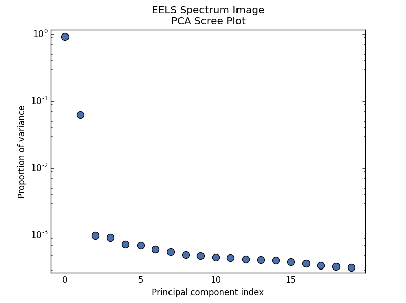
PCA scree plot

New in version 1.2.0: log, threshold, hline, xaxis_type, xaxis_labeling, signal_fmt, noise_fmt, threshold, xaxis_type keyword arguments.

The default options for this method will plot a bare scree plot, but the method’s arguments allow for a great deal of customization. For example, by specifying a threshold value, a cutoff line will be drawn at the total variance specified, and the components above this value will be styled distinctly from the remaining components to show which are considered signal, as opposed to noise. Alternatively, by providing an integer value for threshold, the line will be drawn at the specified component (see below). These options (together with many others), can be customized to develop a figure of your liking. See the documentation of plot_explained_variance_ratio() for more details.

Note that in the above figure, the first component has index 0. This is because Python uses zero based indexing i.e. the initial element of a sequence is found at index 0. To switch to a “number-based” (rather than “index-based”) notation, specify the xaxis_type parameter:

>>> ax = s.plot_explained_variance_ratio(n=20,
...                                      threshold=4,
...                                      xaxis_type='number')

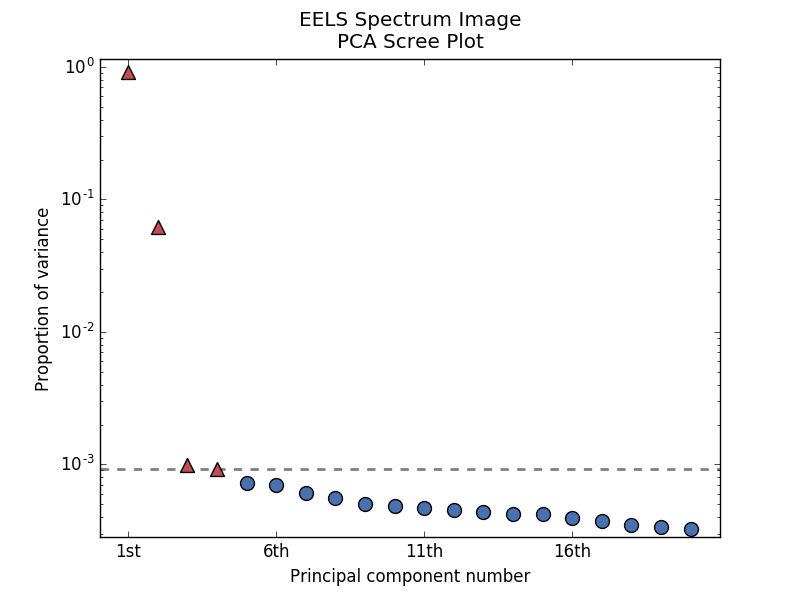
PCA scree plot with number-based axis labeling and a threshold value specified

New in version 0.7.

Sometimes it can be useful to get the explained variance ratio as a spectrum, for example to plot several scree plots obtained using different data pre-treatmentd in the same figure using plot_spectra(). This can be achieved using get_explained_variance_ratio()

Denoising¶

One of the most popular uses of PCA is data denoising. This is achieved by using a limited set of components to make a model of the original, omitting the later components that ideally contain only noise. This is also known as dimensionality reduction.

To perform this operation with HyperSpy, run the get_decomposition_model() method, usually after estimating the dimension of your data using a scree plot. For example:

>>> sc = s.get_decomposition_model(components)

Note

The components argument can be one of several things (None, int, or list of ints):

if None, all the components are used to construct the model.
if int, only the given number of components (starting from index 0) are used to construct the model.
if list of ints, only the components in the given list are used to construct the model.

Sometimes, it is useful to examine the residuals between your original data and the decomposition model. You can easily calculate and display the residuals:

>>> (s - sc).plot()

Hint

Unlike most of the analysis functions, this function returns a new object, which in the example above we have called ‘sc’. You can perform operations on this new object later. It is a copy of the original s object, except that the data has been replaced by the model constructed using the chosen components.

Poissonian noise¶

Many decomposition methods such as PCA assume that the noise of the data follows a Gaussian distribution. In cases where your data is instead corrupted by Poisson noise, HyperSpy can “normalize” the data by performing a scaling operation, which can greatly enhance the result.

To perform Poissonian noise normalization:

>>> # The long way:
>>> s.decomposition(normalize_poissonian_noise=True)

>>> # Because it is the first argument we could have simply written:
>>> s.decomposition(True)

More details about the scaling procedure can be found in [Keenan2004].

Robust principal component analysis¶

PCA is known to be very sensitive to the presence of outliers in data. These outliers can be the result of missing or dead pixels, X-ray spikes, or very low count data. If one assumes a dataset to consist of a low-rank component L corrupted by a sparse error component S, then Robust PCA (RPCA) can be used to recover the low-rank component for subsequent processing [Candes2011].

The default RPCA algorithm is GoDec [Zhou2011]. In HyperSpy it returns the factors and loadings of L, and can be accessed with the following code. You must set the output_dimension when using RPCA.

>>> s.decomposition(algorithm='RPCA_GoDec',
...                 output_dimension=3)

HyperSpy also implements an online algorithm for RPCA developed by Feng et al. [Feng2013]. This minimizes memory usage, making it suitable for large datasets, and can often be faster than the default algorithm.

>>> s.decomposition(algorithm='ORPCA',
...                 output_dimension=3)

The online RPCA implementation sets several default parameters that are usually suitable for most datasets. However, to improve the convergence you can “train” the algorithm with the first few samples of your dataset. For example, the following code will train ORPCA using the first 32 samples of the data.

>>> s.decomposition(algorithm='ORPCA',
...                 output_dimension=3,
...                 training_samples=32)

Finally, online RPCA includes three alternative methods to the default closed-form solver, which can again improve both the convergence and speed of the algorithm. These are particularly useful for very large datasets.

The first method is block-coordinate descent (BCD), and takes no additional parameters:

>>> s.decomposition(algorithm='ORPCA',
...                 output_dimension=3,
...                 method='BCD')

The second is based on stochastic gradient descent (SGD), and takes an additional parameter to set the learning rate. The learning rate dictates the size of the steps taken by the gradient descent algorithm, and setting it too large can lead to oscillations that prevent the algorithm from finding the correct minima. Usually a value between 1 and 2 works well:

>>> s.decomposition(algorithm='ORPCA',
...                 output_dimension=3,
...                 method='SGD',
...                 learning_rate=1.1)

The third method is MomentumSGD, which typically improves the convergence properties of stochastic gradient descent. This takes the further parameter “momentum”, which should be a fraction between 0 and 1.

>>> s.decomposition(algorithm='ORPCA',
...                 output_dimension=3,
...                 method='MomentumSGD',
...                 learning_rate=1.1,
...                 momentum=0.5)

Non-negative matrix factorization¶

Another popular decomposition method is non-negative matrix factorization (NMF), which can be accessed in HyperSpy with:

>>> s.decomposition(algorithm='nmf')

Unlike PCA, NMF forces the components to be strictly non-negative, which can aid the physical interpretation of components for count data such as images, EELS or EDS. For an example of NMF in EELS processing, see [Nicoletti2013].

NMF takes the optional argument “output_dimension”, which determines the number of components to keep. Setting this to a small number is recommended to keep the computation time small. Often it is useful to run a PCA decomposition first and use the scree plot to determine a value for “output_dimension”.

Visualizing results¶

HyperSpy includes a number of plotting methods for the results of decomposition and blind source separation. All the methods begin with plot_:

1 and 4 (new in version 0.7) provide a more compact way of displaying the results. All the other methods display each component in its own window. For 2 and 3 it is wise to provide the number of factors or loadings you wish to visualise, since the default is to plot all of them. For BSS, the default is the number you included when running the blind_source_separation() method. In case of one dimensional factors or loadings, the latter can be toggled on and off by clicking on their corresponding line in the legend.

Obtaining the results as BaseSignal instances¶

New in version 0.7.

The decomposition and BSS results are internally stored as numpy arrays in the BaseSignal class. Frequently it is useful to obtain the decomposition/BSS factors and loadings as HyperSpy signals, and HyperSpy provides the following methods for that purpose:

Saving and loading results¶

There are several methods for storing the result of a machine learning analysis.

Saving in the main file¶

If you save the dataset on which you’ve performed machine learning analysis in the HSpy - HyperSpy’s HDF5 Specification format (the default in HyperSpy) (see Saving data to files), the result of the analysis is also saved in the same file automatically, and it is loaded along with the rest of the data when you next open the file.

Note

This approach currently supports storing one decomposition and one BSS result, which may not be enough for your purposes.

Saving to an external file¶

Alternatively, you can save the results of the current machine learning analysis to a separate file with the save() method:

Save the result of the analysis
>>> s.learning_results.save('my_results')

Load back the results
>>> s.learning_results.load('my_results.npz')

Exporting in different formats¶

It is also possible to export the results of machine learning to any format supported by HyperSpy with:

These methods accept many arguments to customise the way in which the data is exported, so please consult the method documentation. The options include the choice of file format, the prefixes for loadings and factors, saving figures instead of data and more.

Note

Data exported in this way cannot be easily loaded into HyperSpy’s machine learning structure.

Machine learning¶

Introduction¶

Nomenclature¶

Decomposition¶

Principal component analysis¶

Scree plots¶

Denoising¶

Poissonian noise¶

Robust principal component analysis¶

Non-negative matrix factorization¶

Blind Source Separation¶

Visualizing results¶

Obtaining the results as BaseSignal instances¶

Saving and loading results¶

Saving in the main file¶

Saving to an external file¶

Exporting in different formats¶