Fitting the model to the data#

To fit the model to the data at the current coordinates (e.g. to fit one spectrum at a particular point in a spectrum-image), use fit(). HyperSpy implements a number of different optimization approaches, each of which can have particular benefits and/or drawbacks depending on your specific application. A good approach to choosing an optimization approach is to ask yourself the question “Do you want to…”:

Apply bounds to your model parameter values?
Use gradient-based fitting algorithms to accelerate your fit?
Estimate the standard deviations of the parameter values found by the fit?
Fit your data in the least-squares sense, or use another loss function?
Find the global optima for your parameters, or is a local optima acceptable?

Optimization algorithms#

The following table summarizes the features of some of the optimizers currently available in HyperSpy, including whether they support parameter bounds, gradients and parameter error estimation. The “Type” column indicates whether the optimizers find a local or global optima.

Features of supported curve-fitting optimizers.#
Optimizer	Bounds	Gradients	Errors	Loss function	Type	Linear
`"lm"` (default)	Yes	Yes	Yes	Only `"ls"`	local	No
`"trf"`	Yes	Yes	Yes	Only `"ls"`	local	No
`"dogbox"`	Yes	Yes	Yes	Only `"ls"`	local	No
`"odr"`	No	Yes	Yes	Only `"ls"`	local	No
`"lstsq"`	No	No	Yes [1]	Only `"ls"`	global	Yes
`"ridge_regression"`	No	No	Yes [1]	Only `"ls"`	global	Yes
`scipy.optimize.minimize()`	Yes [2]	Yes [2]	No	All	local	No
`"Differential Evolution"`	Yes	No	No	All	global	No
`"Dual Annealing"` [3]	Yes	No	No	All	global	No
`"SHGO"` [3]	Yes	No	No	All	global	No

Footnotes

The default optimizer in HyperSpy is "lm", which stands for the Levenberg-Marquardt algorithm. In earlier versions of HyperSpy (< 1.6) this was known as "leastsq".

Loss functions#

HyperSpy supports a number of loss functions. The default is "ls", i.e. the least-squares loss. For the vast majority of cases, this loss function is appropriate, and has the additional benefit of supporting parameter error estimation and goodness-of-fit testing. However, if your data contains very low counts per pixel, or is corrupted by outliers, the "ML-poisson" and "huber" loss functions may be worth investigating.

Least squares with error estimation#

The following example shows how to perfom least squares optimization with error estimation. First we create data consisting of a line y = a*x + b with a = 1 and b = 100, and we then add Gaussian noise to it:

>>> s = hs.signals.Signal1D(np.arange(100, 300, dtype='float32'))
>>> s.add_gaussian_noise(std=100)

To fit it, we create a model consisting of a Polynomial component of order 1 and fit it to the data.

>>> m = s.create_model()
>>> line = hs.model.components1D.Polynomial(order=1)
>>> m.append(line)
>>> m.fit() 

Once the fit is complete, the optimized value of the parameters and their estimated standard deviation are stored in the following line attributes:

>>> line.a0.value 
0.9924615648843765
>>> line.a1.value 
103.67507406125888
>>> line.a0.std 
0.11771053738516088
>>> line.a1.std 
13.541061301257537

Warning

When the noise is heteroscedastic, only if the metadata.Signal.Noise_properties.variance attribute of the Signal1D instance is defined can the parameter standard deviations be estimated accurately.

If the variance is not defined, the standard deviations are still computed, by setting variance equal to 1. However, this calculation will not be correct unless an accurate value of the variance is provided. See Setting the noise properties for more information.

Weighted least squares with error estimation#

In the following example, we add Poisson noise to the data instead of Gaussian noise, and proceed to fit as in the previous example.

>>> s = hs.signals.Signal1D(np.arange(300))
>>> s.add_poissonian_noise()
>>> m = s.create_model()
>>> line  = hs.model.components1D.Polynomial(order=1)
>>> m.append(line)
>>> m.fit() 
>>> line.a0.value 
-0.7262000522775925
>>> line.a1.value 
1.0086925334859176
>>> line.a0.std 
1.4141418570079
>>> line.a1.std 
0.008185019194679451

Because the noise is heteroscedastic, the least squares optimizer estimation is biased. A more accurate result can be obtained with weighted least squares, where the weights are proportional to the inverse of the noise variance. Although this is still biased for Poisson noise, it is a good approximation in most cases where there are a sufficient number of counts per pixel.

>>> exp_val = hs.signals.Signal1D(np.arange(300)+1)
>>> s.estimate_poissonian_noise_variance(expected_value=exp_val)
>>> line.estimate_parameters(s, 10, 250)
True
>>> m.fit() 
>>> line.a0.value 
-0.6666008600519397
>>> line.a1.value 
1.017145603577098
>>> line.a0.std 
0.8681360488613021
>>> line.a1.std 
0.010308732161043038

Warning

When the attribute metadata.Signal.Noise_properties.variance is defined, the behaviour is to perform a weighted least-squares fit using the inverse of the noise variance as the weights. In this scenario, to then disable weighting, you will need to unset the attribute. You can achieve this with set_noise_variance():

>>> m.signal.set_noise_variance(None) # This will now be an unweighted fit
>>> m.fit() 
>>> line.a0.value 
-1.9711403542163477
>>> line.a1.value 
1.0258716193502546

Poisson maximum likelihood estimation#

To avoid biased estimation in the case of data corrupted by Poisson noise with very few counts, we can use Poisson maximum likelihood estimation (MLE) instead. This is an unbiased estimator for Poisson noise. To perform MLE, we must use a general, non-linear optimizer from the table above, such as Nelder-Mead or L-BFGS-B:

>>> m.fit(optimizer="Nelder-Mead", loss_function="ML-poisson") 
>>> line.a0.value 
0.00025567973144090695
>>> line.a1.value 
1.0036866523183754

Estimation of the parameter errors is not currently supported for Poisson maximum likelihood estimation.

Huber loss function#

HyperSpy also implements the Huber loss function, which is typically less sensitive to outliers in the data compared to the least-squares loss. Again, we need to use one of the general non-linear optimization algorithms:

>>> m.fit(optimizer="Nelder-Mead", loss_function="huber") 

Estimation of the parameter errors is not currently supported for the Huber loss function.

Custom loss functions#

As well as the built-in loss functions described above, a custom loss function can be passed to the model:

>>> def my_custom_function(model, values, data, weights=None):
...    """
...    Parameters
...    ----------
...    model : Model instance
...        the model that is fitted.
...    values : np.ndarray
...        A one-dimensional array with free parameter values suggested by the
...        optimizer (that are not yet stored in the model).
...    data : np.ndarray
...        A one-dimensional array with current data that is being fitted.
...    weights : {np.ndarray, None}
...        An optional one-dimensional array with parameter weights.
...
...    Returns
...    -------
...    score : float
...        A signle float value, representing a score of the fit, with
...        lower values corresponding to better fits.
...    """
...    # Almost any operation can be performed, for example:
...    # First we store the suggested values in the model
...    model.fetch_values_from_array(values)
...
...    # Evaluate the current model
...    cur_value = model(onlyactive=True)
...
...    # Calculate the weighted difference with data
...    if weights is None:
...        weights = 1
...    difference = (data - cur_value) * weights
...
...    # Return squared and summed weighted difference
...    return (difference**2).sum()

>>> # We must use a general non-linear optimizer
>>> m.fit(optimizer='Nelder-Mead', loss_function=my_custom_function) 

If the optimizer requires an analytical gradient function, it can be similarly passed, using the following signature:

>>> def my_custom_gradient_function(model, values, data, weights=None):
...    """
...    Parameters
...    ----------
...    model : Model instance
...        the model that is fitted.
...    values : np.ndarray
...        A one-dimensional array with free parameter values suggested by the
...        optimizer (that are not yet stored in the model).
...    data : np.ndarray
...        A one-dimensional array with current data that is being fitted.
...    weights : {np.ndarray, None}
...        An optional one-dimensional array with parameter weights.
...
...    Returns
...    -------
...    gradients : np.ndarray
...        a one-dimensional array of gradients, the size of `values`,
...        containing each parameter gradient with the given values
...    """
...    # As an example, estimate maximum likelihood gradient:
...    model.fetch_values_from_array(values)
...    cur_value = model(onlyactive=True)
...
...    # We use in-built jacobian estimation
...    jac = model._jacobian(values, data)
...
...    return -(jac * (data / cur_value - 1)).sum(1)

>>> # We must use a general non-linear optimizer again
>>> m.fit(optimizer='L-BFGS-B',
...       loss_function=my_custom_function,
...       grad=my_custom_gradient_function) 

Using gradient information#

New in version 1.6: grad="analytical" and grad="fd" keyword arguments

Optimization algorithms that take into account the gradient of the loss function will often out-perform so-called “derivative-free” optimization algorithms in terms of how rapidly they converge to a solution. HyperSpy can use analytical gradients for model-fitting, as well as numerical estimates of the gradient based on finite differences.

If all the components in the model support analytical gradients, you can pass grad="analytical" in order to use this information when fitting. The results are typically more accurate than an estimated gradient, and the optimization often runs faster since fewer function evaluations are required to calculate the gradient.

Following the above examples:

>>> m = s.create_model()
>>> line = hs.model.components1D.Polynomial(order=1)
>>> m.append(line)

>>> # Use a 2-point finite-difference scheme to estimate the gradient
>>> m.fit(grad="fd", fd_scheme="2-point") 

>>> # Use the analytical gradient
>>> m.fit(grad="analytical") 

>>> # Huber loss and Poisson MLE functions
>>> # also support analytical gradients
>>> m.fit(grad="analytical", loss_function="huber") 
>>> m.fit(grad="analytical", loss_function="ML-poisson") 

Note

Analytical gradients are not yet implemented for the Model2D class.

Bounded optimization#

Non-linear optimization can sometimes fail to converge to a good optimum, especially if poor starting values are provided. Problems of ill-conditioning and non-convergence can be improved by using bounded optimization.

All components’ parameters have the attributes parameter.bmin and parameter.bmax (“bounded min” and “bounded max”). When fitting using the bounded=True argument by m.fit(bounded=True) or m.multifit(bounded=True), these attributes set the minimum and maximum values allowed for parameter.value.

Currently, not all optimizers support bounds - see the table above. In the following example, a Gaussian histogram is fitted using a Gaussian component using the Levenberg-Marquardt (“lm”) optimizer and bounds on the centre parameter.

>>> s = hs.signals.BaseSignal(np.random.normal(loc=10, scale=0.01,
... size=100000)).get_histogram()
>>> s.axes_manager[-1].is_binned = True
>>> m = s.create_model()
>>> g1 = hs.model.components1D.Gaussian()
>>> m.append(g1)
>>> g1.centre.value = 7
>>> g1.centre.bmin = 7
>>> g1.centre.bmax = 14
>>> m.fit(optimizer="lm", bounded=True) 
>>> m.print_current_values() 
Model1D:  histogram
Gaussian: Gaussian
Active: True
Parameter Name |  Free |      Value |        Std |        Min |        Max
============== | ===== | ========== | ========== | ========== | ==========
             A |  True | 99997.3481 | 232.333693 |        0.0 |       None
         sigma |  True | 0.00999184 | 2.68064163 |       None |       None
        centre |  True | 9.99980788 | 2.68064070 |        7.0 |       14.0

Linear least squares#

New in version 1.7.

Linear fitting can be used to address some of the drawbacks of non-linear optimization:

it doesn’t suffer from the starting parameters issue, which can sometimes be problematic with nonlinear fitting. Since linear fitting uses linear algebra to find the solution (find the parameter values of the model), the solution is a unique solution, while nonlinear optimization uses an iterative approach and therefore relies on the initial values of the parameters.
it is fast, because i) in favorable situations, the signal can be fitted in a vectorized fashion, i.e. the signal is fitted in a single run instead of iterating over the navigation dimension; ii) it is not iterative, i.e. it does the calculation only one time instead of 10-100 iterations, depending on how quickly the non-linear optimizer will converge.

However, linear fitting can only fit linear models and will not be able to fit parameters which vary non-linearly.

A component is considered linear when its free parameters scale the component only in the y-axis. For the exemplary function y = a*x**b, a is a linear parameter, whilst b is not. If b.free = False, then the component is linear. Components can also be made up of several linear parts. For instance, the 2D-polynomial y = a*x**2+b*y**2+c*x+d*y+e is entirely linear.

Note

After creating a model with values for the nonlinear parameters, a quick way to set all nonlinear parameters to be free = False is to use m.set_parameters_not_free(only_nonlinear=True)

To check if a parameter is linear, use the model or component method print_current_values(). For a component to be considered linear, it can hold only one free parameter, and that parameter must be linear.

If all components in a model are linear, then a linear optimizer can be used to solve the problem as a linear regression problem! This can be done using two approaches:

the standard pixel-by-pixel approach as used by the nonlinear optimizers
fit the entire dataset in one vectorised operation, which will be much faster (up to 1000 times). However, there is a caveat: all fixed parameters must have the same value across the dataset in order to avoid creating a very large array whose size will scale with the number of different values of the non-free parameters.

Note

A good example of a linear model in the electron-microscopy field is an Energy-Dispersive X-ray Spectroscopy (EDS) dataset, which typically consists of a polynomial background and Gaussian peaks with well-defined energy (Gaussian.centre) and peak widths (Gaussian.sigma). This dataset can be fit extremely fast with a linear optimizer.

There are two implementations of linear least squares fitting in hyperspy:

the 'lstsq' optimizer, which uses numpy.linalg.lstsq(), or dask.array.linalg.lstsq() for lazy signals.
the 'ridge_regression' optimizer, which supports regularization (see sklearn.linear_model.Ridge for arguments to pass to fit()), but does not support lazy signals.

As for non-linear least squares fitting, weighted least squares is supported.

In the following example, we first generate a 300x300 navigation signal of varying total intensity, and then populate it with an EDS spectrum at each point. The signal can be fitted with a polynomial background and a Gaussian for each peak. Hyperspy automatically adds these to the model, and fixes the centre and sigma parameters to known values. Fitting this model with a non-linear optimizer can about half an hour on a decent workstation. With a linear optimizer, it takes seconds.

>>> nav = hs.signals.Signal2D(np.random.random((300, 300))).T
>>> s = exspy.data.EDS_TEM_FePt_nanoparticles() * nav 
>>> m = s.create_model() 

>>> m.multifit(optimizer='lstsq') 

Standard errors for the parameters are by default not calculated when the dataset is fitted in vectorized fashion, because it has large memory requirement. If errors are required, either pass calculate_errors=True as an argument to multifit(), or rerun multifit() with a nonlinear optimizer, which should run fast since the parameters are already optimized.

None of the linear optimizers currently support bounds.

Optimization results#

After fitting the model, details about the optimization procedure, including whether it finished successfully, are returned as scipy.optimize.OptimizeResult object, according to the keyword argument return_info=True. These details are often useful for diagnosing problems such as a poorly-fitted model or a convergence failure. You can also access the object as the fit_output attribute:

>>> m.fit() 
>>> type(m.fit_output) 
<scipy.optimize.OptimizeResult object>

You can also print this information using the print_info keyword argument:

# Print the info to stdout
>>> m.fit(optimizer="L-BFGS-B", print_info=True) # doctest: +SKIP
Fit info:
  optimizer=L-BFGS-B
  loss_function=ls
  bounded=False
  grad="fd"
Fit result:
  hess_inv: <3x3 LbfgsInvHessProduct with dtype=float64>
   message: b'CONVERGENCE: REL_REDUCTION_OF_F_<=_FACTR*EPSMCH'
      nfev: 168
       nit: 32
      njev: 42
    status: 0
   success: True
         x: array([ 9.97614503e+03, -1.10610734e-01,  1.98380701e+00])

Goodness of fit#

The chi-squared, reduced chi-squared and the degrees of freedom are computed automatically when fitting a (weighted) least-squares model (i.e. only when loss_function="ls"). They are stored as signals, in the chisq, red_chisq and dof attributes of the model respectively.

Warning

Unless metadata.Signal.Noise_properties.variance contains an accurate estimation of the variance of the data, the chi-squared and reduced chi-squared will not be computed correctly. This is true for both homocedastic and heteroscedastic noise.

Visualizing the model#

To visualise the result use the plot() method:

>>> m.plot() # Visualise the results

By default only the full model line is displayed in the plot. In addition, it is possible to display the individual components by calling enable_plot_components() or directly using plot():

>>> m.plot(plot_components=True) # Visualise the results

To disable this feature call disable_plot_components().

New in version 1.4: plot() keyword arguments

All extra keyword arguments are passed to the plot() method of the corresponding signal object. The following example plots the model signal figure but not its navigator:

>>> m.plot(navigator=False)

By default the model plot is automatically updated when any parameter value changes. It is possible to suspend this feature with suspend_update().

Setting the initial parameters#

Non-linear optimization often requires setting sensible starting parameters. This can be done by plotting the model and adjusting the parameters by hand.

Changed in version 1.3: All notebook_interaction methods renamed to gui(). The notebook_interaction methods were removed in 2.0.

If running in a Jupyter Notebook, interactive widgets can be used to conveniently adjust the parameter values by running gui() for BaseModel, Component and Parameter.

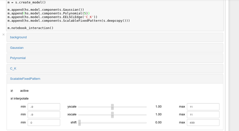
../../_images/notebook_widgets.png — Interactive widgets for the full model in a Jupyter notebook. Drag the sliders to adjust current parameter values. Typing different minimum and maximum values changes the boundaries of the slider.#

Also, enable_adjust_position() provides an interactive way of setting the position of the components with a well-defined position. disable_adjust_position() disables the tool.

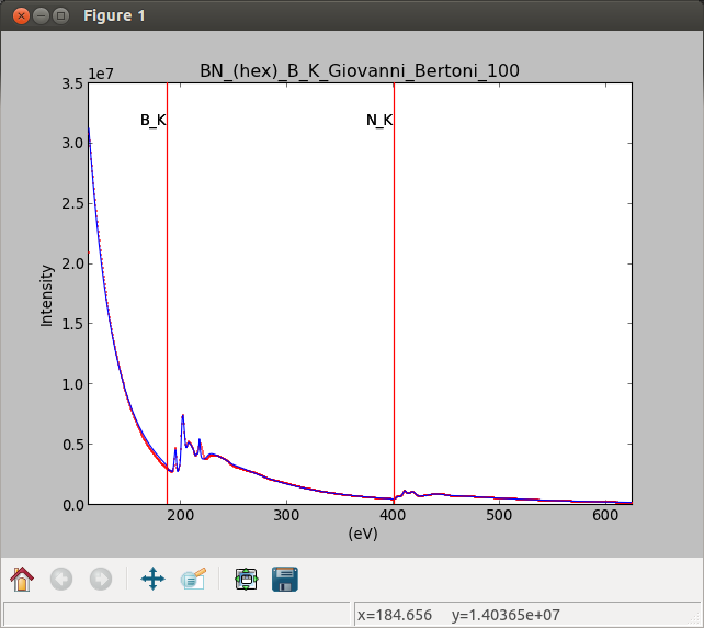
../../_images/model_adjust_position.png — Interactive component position adjustment tool. Drag the vertical lines to set the initial value of the position parameter.#

Exclude data from the fitting process#

The following BaseModel methods can be used to exclude undesired spectral channels from the fitting process:

The example below shows how a boolean array can be easily created from the signal and how the isig syntax can be used to define the signal range.

>>> # Create a sample 2D gaussian dataset
>>> g = hs.model.components2D.Gaussian2D(
...   A=1, centre_x=-5.0, centre_y=-5.0, sigma_x=1.0, sigma_y=2.0,)

>>> scale = 0.1
>>> x = np.arange(-10, 10, scale)
>>> y = np.arange(-10, 10, scale)
>>> X, Y = np.meshgrid(x, y)

>>> im = hs.signals.Signal2D(g.function(X, Y))
>>> im.axes_manager[0].scale = scale
>>> im.axes_manager[0].offset = -10
>>> im.axes_manager[1].scale = scale
>>> im.axes_manager[1].offset = -10

>>> m = im.create_model() # Model initialisation
>>> gt = hs.model.components2D.Gaussian2D()
>>> m.append(gt)

>>> m.set_signal_range(-7, -3, -9, -1) # Set signal range
>>> m.fit() 

Alternatively, create a boolean signal of the same shape
as the signal space of im

>>> signal_mask = im > 0.01

>>> m.set_signal_range_from_mask(signal_mask.data) # Set signal range
>>> m.fit() 

Fitting multidimensional datasets#

To fit the model to all the elements of a multidimensional dataset, use multifit():

>>> m.multifit() # warning: this can be a lengthy process on large datasets

multifit() fits the model at the first position, stores the result of the fit internally and move to the next position until reaching the end of the dataset.

Note

Sometimes this method can fail, especially in the case of a TEM spectrum image of a particle surrounded by vacuum (since in that case the top-left pixel will typically be an empty signal).

To get sensible starting parameters, you can do a single fit() after changing the active position within the spectrum image (either using the plotting GUI or by directly modifying s.axes_manager.indices as in Setting axis properties).

After doing this, you can initialize the model at every pixel to the values from the single pixel fit using m.assign_current_values_to_all(), and then use multifit() to perform the fit over the entire spectrum image.

New in version 1.6: New optional fitting iteration path “serpentine”

New in version 2.0: New default iteration path for fitting is “serpentine”`

In HyperSpy, curve fitting on a multidimensional dataset happens in the following manner: Pixels are fit along the row from the first index in the first row, and once the last pixel in the row is reached, one proceeds in reverse order from the last index in the second row. This procedure leads to a serpentine pattern, as seen on the image below. The serpentine pattern supports n-dimensional navigation space, so the first index in the second frame of a three-dimensional navigation space will be at the last position of the previous frame.

An alternative scan pattern would be the 'flyback' scheme, where the map is iterated through row by row, always starting from the first index. This pattern can be explicitly set using the multifit() iterpath='flyback' argument. However, the 'serpentine' strategy is usually more robust, as it always moves on to a neighbouring pixel and the fitting procedure uses the fit result of the previous pixel as the starting point for the next. A common problem in the 'flyback' pattern is that the fitting fails going from the end of one row to the beginning of the next, as the spectrum can change abruptly.

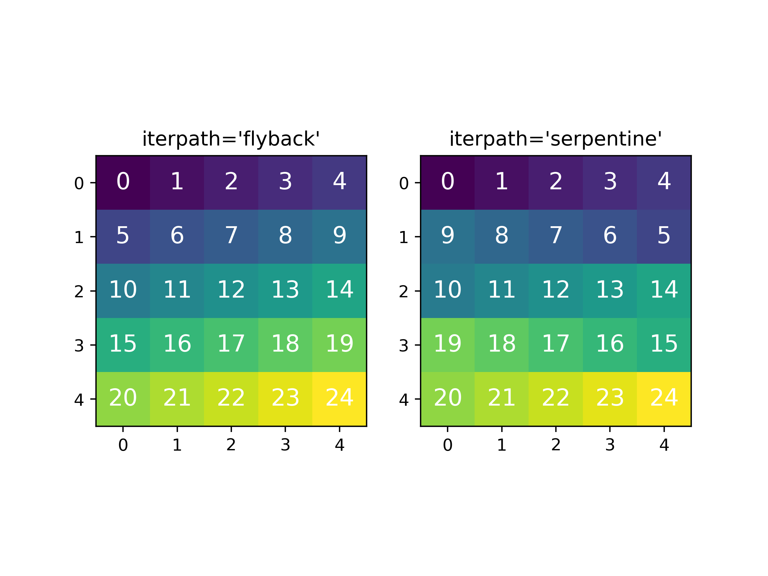
../../_images/FlybackVsSerpentine.png — Comparing the scan patterns generated by the `'flyback'` and `'serpentine'` iterpath options for a 2D navigation space. The pixel intensity and number refers to the order that the signal is fitted in.#

In addition to 'serpentine' and 'flyback', iterpath can take as argument any list or array of indices, or a generator of such, as explained in the Iterating AxesManager section.

Sometimes one may like to store and fetch the value of the parameters at a given position manually. This is possible using store_current_values() and fetch_stored_values().

Visualising the result of the fit#

The BaseModel plot_results(), Component plot() and Parameter plot() methods can be used to visualise the result of the fit when fitting multidimensional datasets.