Fourier ratio deconvolution

This example demonstrates how to perform Fourier ratio deconvolution on Mn L_2,3 core-loss edge.

import hyperspy.api as hs

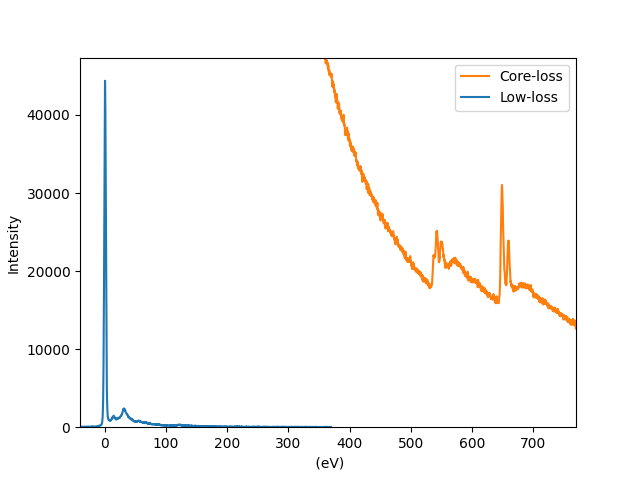
Load a core-loss and low-loss EELS spectra and align the zero-loss peak. The core-loss spectrum contains the O K edge at 532 eV and the Mn L_2,3 edgeat 640 eV.

low_loss = hs.load("../lowloss_spectrum.msa", signal_type="EELS")
core_loss = hs.load("../coreloss_spectrum.msa", signal_type="EELS")

low_loss.align_zero_loss_peak(also_align=core_loss)

hs.plot.plot_spectra([low_loss, core_loss], legend=["Low-loss", "Core-loss"])

Initial ZLP position statistics
-------------------------------
Summary statistics
------------------
mean:   0.8
std:    0

min:    0.8
Q1:     0.8
median: 0.8
Q3:     0.8
max:    0.8

<Axes: xlabel=' (eV)', ylabel='Intensity'>

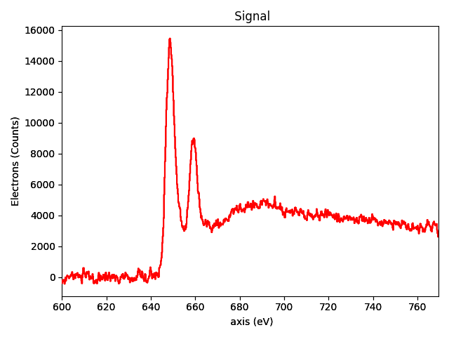
Remove the background from the Mn L_2,3 edge.

Mn_edge = core_loss.remove_background([600.0, 638.0]).isig[600.0:]
Mn_edge.plot()

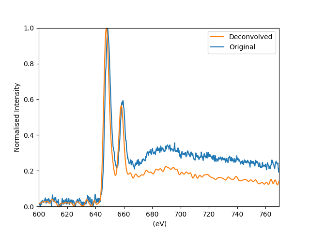
Then perform Fourier ratio deconvolution using the low-loss spectrum as the reference.

Mn_edge_deconv = Mn_edge.fourier_ratio_deconvolution(low_loss=low_loss)

  0%|          | 0/2 [00:00<?, ?it/s]
100%|██████████| 2/2 [00:00<00:00, 3515.76it/s]

Plot the original and deconvolved spectra.

hs.plot.plot_spectra(
    [Mn_edge, Mn_edge_deconv], legend=["Original", "Deconvolved"], normalise=True
)

<Axes: xlabel=' (eV)', ylabel='Normalised Intensity'>

sphinx_gallery_thumbnail_number = 3