Signal1D Tools#
The methods described in this section are only available for one-dimensional signals in the Signal1D class.
Cropping#
The crop_signal() crops the
the signal object along the signal axis (e.g. the spectral energy range)
in-place. If no parameter is passed, a user interface
appears in which to crop the one dimensional signal. For example:
>>> s = hs.data.two_gaussians()
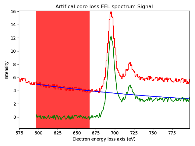
>>> s.crop_signal(5, 15) # s is cropped in place
Additionally, cropping in HyperSpy can be performed using the Signal indexing syntax. For example, the following crops a signal to the 5.0-15.0 region:
>>> s = hs.data.two_gaussians()
>>> sc = s.isig[5.:15.] # s is not cropped, sc is a "cropped view" of s
It is possible to crop interactively using Region Of Interest (ROI). For example:
>>> s = hs.data.two_gaussians()
>>> roi = hs.roi.SpanROI(left=5, right=15)
>>> s.plot()
>>> sc = roi.interactive(s)
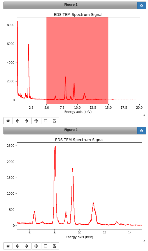
Interactive spectrum cropping using a ROI.#
Background removal#
Added in version 1.4: zero_fill and plot_remainder keyword arguments and big speed
improvements.
The remove_background() method provides
background removal capabilities through both a CLI and a GUI. Selected components
from components1D are fitted in a given range to estimate the
background and substract it from the signals.
The GUI displays an interactive preview of the remainder after background subtraction.
Currently, the following background types are supported: Doniach, Exponential, Gaussian,
Lorentzian, Polynomial, Power law (default), Offset, Skew normal, Split Voigt
and Voigt. By default, the background parameters are estimated using analytical
approximations (keyword argument fast=True). The fast option is not accurate
for most background types - except Gaussian, Offset and Power law -
but it is useful to estimate the initial fitting parameters before performing a
full fit. For better accuracy, but higher processing time, the parameters can
be estimated using curve fitting by setting fast=False.
Example of usage:
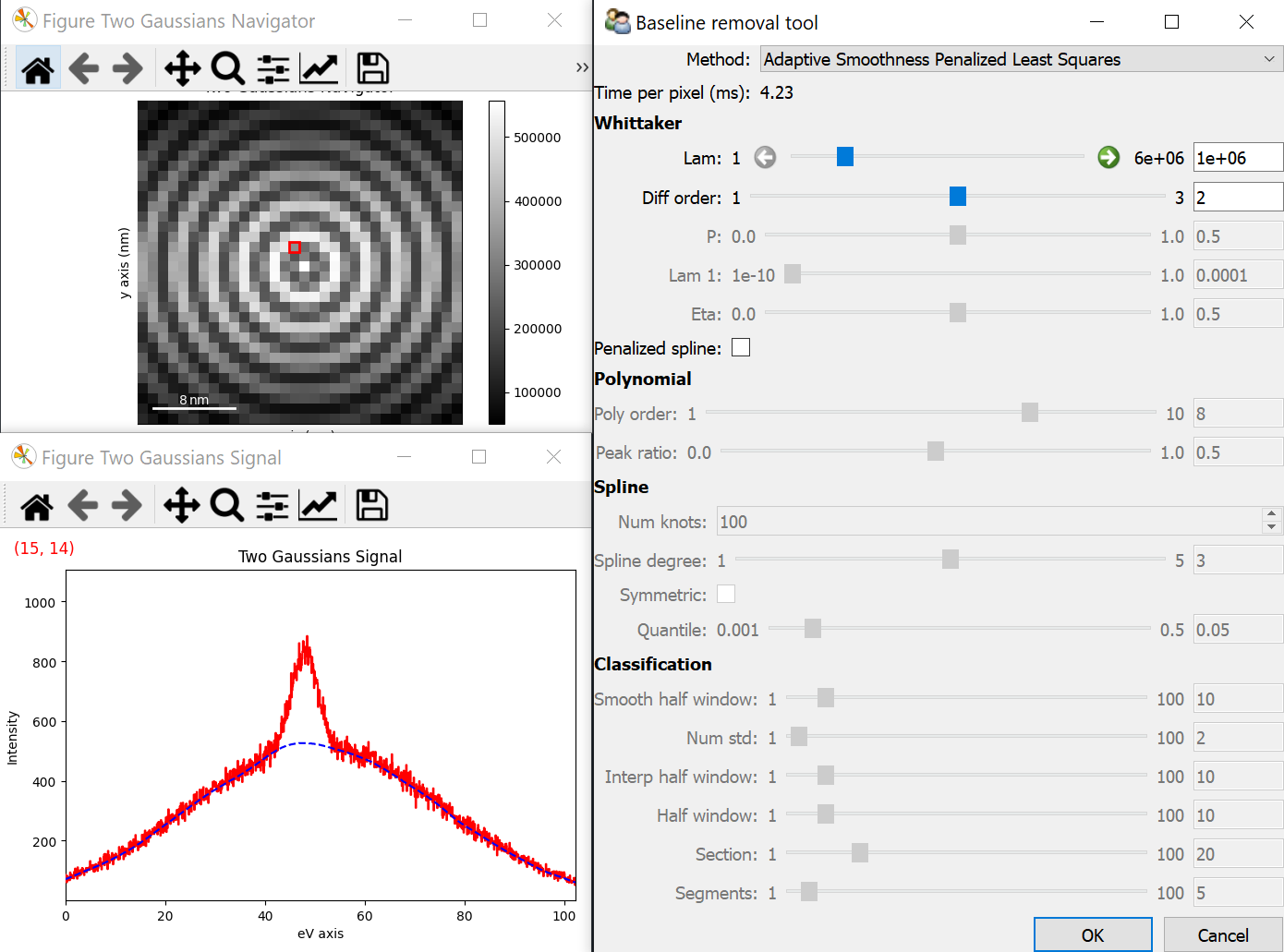
>>> s = exspy.data.EELS_MnFe(add_powerlaw=True)
>>> s.remove_background()
Interactive background removal. In order to select the region used to estimate the background parameters (red area in the figure) click inside the axes of the figure and drag to the right without releasing the button.#
Baseline removal#
Added in version 2.3.
The remove_baseline() method provides baseline
removal capabilities through both a CLI and a GUI. The baseline is estimated using
methods implemented in pybaselines.
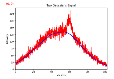
>>> s = hs.data.two_gaussians()
>>> s.remove_baseline()
Interactive baseline removal. The estimated baseline is shown as a blue dash in the signal plot. The GUI allows selecting the method and the main parameters.#
Example using remove_baseline()#
Calibration#
The calibrate() method provides a user
interface to calibrate the spectral axis.
Alignment#
The following methods use sub-pixel cross-correlation or user-provided shifts to align spectra. They support applying the same transformation to multiple files.
Integration#
To integrate signals use the integrate1D() method.
Possibly in combination with a Region Of Interest (ROI) if interactivity is required.
Otherwise, a signal subrange for integration can also be chosen with the
isig method.
>>> s.isig[0.2:0.5].integrate1D(axis=0)
Data smoothing#
The following methods (that include user interfaces when no arguments are passed) can perform data smoothing with different algorithms:
smooth_lowess()(requiresstatsmodelsto be installed)
Peak finding#
A peak finding routine based on the work of T. O’Haver is available in HyperSpy
through the find_peaks1D_ohaver()
method.
Estimate peak width#
For asymmetric peaks, fitted functions may not provide
an accurate description of the peak, in particular the peak width. The function
estimate_peak_width()
determines the width of a peak at a certain fraction of its maximum value.
Other methods#
Interpolate the spectra in between two positions
interpolate_in_between()Convolve the spectra with a gaussian
gaussian_filter()Apply a hanning taper to the spectra
hanning_taper()