Signal2D Tools#
The methods described in this section are only available for two-dimensional
signals in the Signal2D. class.
Signal registration and alignment#
The align2D() and
estimate_shift2D() methods provide
advanced image alignment functionality.
# Estimate shifts, then align the images
>>> shifts = s.estimate_shift2D() # doctest: +SKIP
>>> s.align2D(shifts=shifts) # doctest: +SKIP

# Estimate and align in a single step
>>> s.align2D() # doctest: +SKIP
Warning
s.align2D() will modify the data in-place. If you don’t want
to modify your original data, first take a copy before aligning.
Sub-pixel accuracy can be achieved in two ways:
scikit-image’s upsampled matrix-multiplication DFT method [Guizar2008], by setting the
sub_pixel_factorkeyword argumentfor multi-dimensional datasets only, using the statistical method [Schaffer2004], by setting the
referencekeyword argument to"stat"
# skimage upsampling method
>>> shifts = s.estimate_shift2D(sub_pixel_factor=20) # doctest: +SKIP

# stat method
>>> shifts = s.estimate_shift2D(reference="stat") # doctest: +SKIP

# combined upsampling and statistical method
>>> shifts = s.estimate_shift2D(reference="stat", sub_pixel_factor=20) # doctest: +SKIP
If you have a large stack of images, the image alignment is automatically done in parallel.
You can control the number of threads used with the num_workers argument. Or by adjusting
the scheduler.
# Estimate shifts
>>> shifts = s.estimate_shift2D() # doctest: +SKIP

# Align images in parallel using 4 threads
>>> s.align2D(shifts=shifts, num_workers=4) # doctest: +SKIP
Cropping a Signal2D#
The crop_signal() method crops the
image in-place e.g.:
>>> im = hs.data.wave_image()
>>> im.crop_signal(left=0.5, top=0.7, bottom=2.0) # im is cropped in-place
Cropping in HyperSpy is performed using the Signal indexing syntax. For example, to crop an image:
>>> im = hs.data.wave_image()
>>> # im is not cropped, imc is a "cropped view" of im
>>> imc = im.isig[0.5:, 0.7:2.0]
It is possible to crop interactively using Region Of Interest (ROI). For example:
>>> im = hs.data.wave_image()
>>> roi = hs.roi.RectangularROI()
>>> im.plot()
>>> imc = roi.interactive(im)
>>> imc.plot()
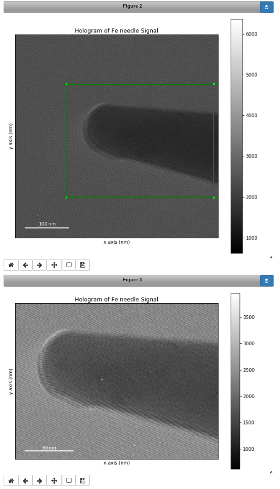
Interactive image cropping using a ROI.#
Interactive calibration#
The scale can be calibrated interactively by using
calibrate(), which is used to
set the scale by dragging a line across some feature of known size.
>>> s = hs.signals.Signal2D(np.random.random((200, 200)))
>>> s.calibrate()
The same function can also be used non-interactively.
>>> s = hs.signals.Signal2D(np.random.random((200, 200)))
>>> s.calibrate(x0=1, y0=1, x1=5, y1=5, new_length=3.4, units="nm", interactive=False)
Add a linear ramp#
A linear ramp can be added to the signal via the
add_ramp() method. The parameters
ramp_x and ramp_y dictate the slope of the ramp in x- and y direction,
while the offset is determined by the offset parameter. The fulcrum of the
linear ramp is at the origin and the slopes are given in units of the axis
with the according scale taken into account. Both are available via the
AxesManager of the signal.
Peak finding#
Added in version 1.6.
The find_peaks() method provides access
to a number of algorithms for peak finding in two dimensional signals. The
methods available are:
Maximum based peak finder#
>>> s.find_peaks(method='local_max')
>>> s.find_peaks(method='max')
>>> s.find_peaks(method='minmax')
These methods search for peaks using maximum (and minimum) values in the
image. There all have a distance parameter to set the minimum distance
between the peaks.
the
'local_max'method uses theskimage.feature.peak_local_max()function (distanceandthresholdparameters are mapped tomin_distanceandthreshold_abs, respectively).the
'max'method uses thefind_peaks_max()function to search for peaks higher thanalpha * sigma, wherealphais parameters andsigmais the standard deviation of the image. It also has adistanceparameters to set the minimum distance between peaks.the
'minmax'method uses thefind_peaks_minmax()function to locate the positive peaks in an image by comparing maximum and minimum filtered images. Itsthresholdparameter defines the minimum difference between the maximum and minimum filtered images.
Zaeferrer peak finder#
>>> s.find_peaks(method='zaefferer')
This algorithm was developed by Zaefferer [Zaefferer2000].
It is based on a gradient threshold followed by a local maximum search within a square window,
which is moved until it is centered on the brightest point, which is taken as a
peak if it is within a certain distance of the starting point. It uses the
find_peaks_zaefferer() function, which can take
grad_threshold, window_size and distance_cutoff as parameters. See
the find_peaks_zaefferer() function documentation
for more details.
Ball statistical peak finder#
>>> s.find_peaks(method='stat')
Described by White [White2009], this method is based on finding points that
have a statistically higher value than the surrounding areas, then iterating
between smoothing and binarising until the number of peaks has converged. This
method can be slower than the others, but is very robust to a variety of image types.
It uses the find_peaks_stat() function, which can take
alpha, window_radius and convergence_ratio as parameters. See the
find_peaks_stat() function documentation for more
details.
Matrix based peak finding#
>>> s.find_peaks(method='laplacian_of_gaussians')
>>> s.find_peaks(method='difference_of_gaussians')
These methods are essentially wrappers around the
Laplacian of Gaussian (skimage.feature.blob_log()) or the difference
of Gaussian (skimage.feature.blob_dog()) methods, based on stacking
the Laplacian/difference of images convolved with Gaussian kernels of various
standard deviations. For more information, see the example in the
scikit-image documentation.
Template matching#
>>> x, y = np.meshgrid(np.arange(-2, 2.5, 0.5), np.arange(-2, 2.5, 0.5))
>>> template = hs.model.components2D.Gaussian2D().function(x, y)
>>> s.find_peaks(method='template_matching', template=template, interactive=False)
<BaseSignal, title: , dimensions: (|ragged)>
This method locates peaks in the cross correlation between the image and a
template using the find_peaks_xc() function. See
the find_peaks_xc() function documentation for
more details.
Interactive parametrization#
Many of the peak finding algorithms implemented here have a number of tunable parameters that significantly affect their accuracy and speed. The GUIs can be used to set to select the method and set the parameters interactively:
>>> s.find_peaks(interactive=True)
Several widgets are available:
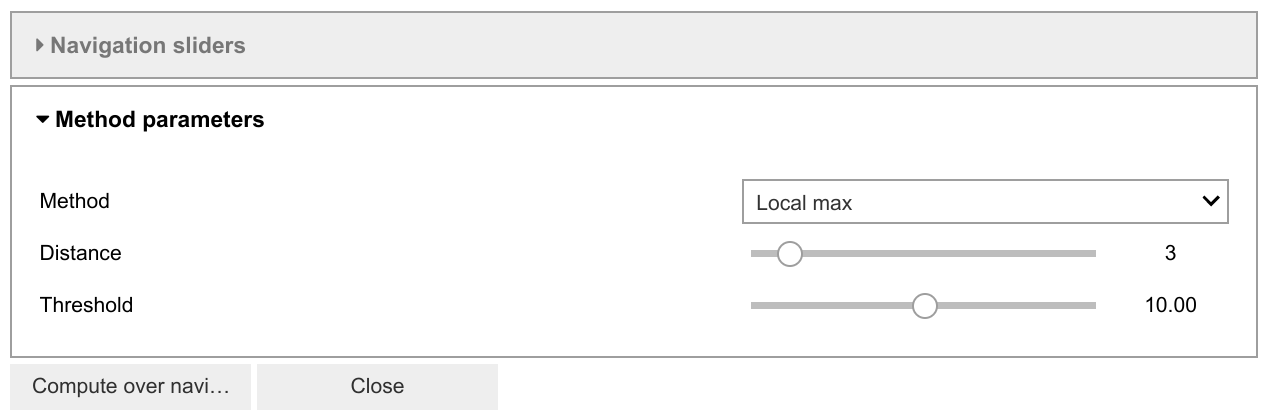
The method selector is used to compare different methods. The last-set parameters are maintained.
The parameter adjusters will update the parameters of the method and re-plot the new peaks.
Note
Some methods take significantly longer than others, particularly where there are a large number of peaks to be found. The plotting window may be inactive during this time.