Electron Energy Loss Spectroscopy

Tools for EELS data analysis

The functions described in this chapter are only available for the EELSSpectrum class. To transform a BaseSignal (or subclass) into a EELSSpectrum:

>>> s.set_signal_type("EELS")

Note these chapter discusses features that are available only for EELSSpectrum class. However, this class inherits many useful feature from its parent class that are documented in previous chapters.

Elemental composition of the sample

It can be useful to define the elemental composition of the sample for archiving purposes or to use some feature (e.g. curve fitting) that requires this information. The elemental composition of the sample can be declared using add_elements(). The information is stored in the metadata attribute (see Metadata structure). This information is saved to file when saving in the hspy format (HyperSpy’s HDF5 specification).

An utility function get_edges_near_energy() can be helpful to identify possible elements in the sample. get_edges_near_energy() returns a list of edges arranged in the order closest to the specified energy within a window, both measured in eV. The size of the window can be controlled by the argument width (default as 10)— If the specified energy is 849 eV and the width is 6 eV, it returns a list of edges with onset energy between 846 eV to 852 eV and they are arranged in the order closest to 849 eV.

>>> from hyperspy.misc.eels.tools import get_edges_near_energy
>>> get_edges_near_energy(532)
['O_K', 'Pd_M3', 'Sb_M5', 'Sb_M4']
>>> get_edges_near_energy(849, width=6)
['La_M4', 'Fe_L1']

` The static method print_edges_near_energy() in EELSSpectrum will print out a table containing more information about the edges.

>>> s = hs.datasets.artificial_data.get_core_loss_eels_signal()
>>> s.print_edges_near_energy(401, width=20)
+-------+-------------------+-----------+-----------------------------+
|  edge | onset energy (eV) | relevance |         description         |
+-------+-------------------+-----------+-----------------------------+
|  N_K  |       401.0       |   Major   |         Abrupt onset        |
| Sc_L3 |       402.0       |   Major   | Sharp peak. Delayed maximum |
| Cd_M5 |       404.0       |   Major   |       Delayed maximum       |
| Sc_L2 |       407.0       |   Major   | Sharp peak. Delayed maximum |
| Mo_M2 |       410.0       |   Minor   |          Sharp peak         |
| Mo_M3 |       392.0       |   Minor   |          Sharp peak         |
| Cd_M4 |       411.0       |   Major   |       Delayed maximum       |
+-------+-------------------+-----------+-----------------------------+

The method edges_at_energy() allows inspecting different sections of the signal for interactive edge identification (the default). A region can be selected by dragging the mouse across the signal and after clicking the Update button, edges with onset energies within the selected energy range will be displayed. By toggling the edge buttons, it will put or remove the corresponding edges on the signal. When the Complementary edge box is ticked, edges outside the selected range with the same element of edges within the selected energy range will be shown as well to aid identification of edges.

>>> s = hs.datasets.artificial_data.get_core_loss_eels_signal()
>>> s.edges_at_energy()

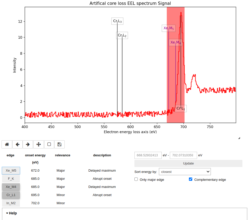
Labels of edges can be put or remove by toggling the edge buttons.

Thickness estimation

New in version 1.6: Option to compute the absolute thickness, including the angular corrections and mean free path estimation.

The estimate_thickness() method can estimate the thickness from a low-loss EELS spectrum using the log-ratio method. If the beam energy, collection angle, convergence angle and sample density are known, the absolute thickness is computed using the method in [Iakoubovskii2008]. This includes the estimation of the inelastic mean free path (iMFP). For more accurate results, it is possible to input the iMFP of the material if known. If the density and/or the iMFP are not known, the output is the thickness relative to the (unknown) iMFP without any angular corrections.

Zero-loss peak centre and alignment

The estimate_zero_loss_peak_centre() can be used to estimate the position of the zero-loss peak. The method assumes that the ZLP is the most intense feature in the spectra. For a more general approach see find_peaks1D_ohaver().

The align_zero_loss_peak() can align the ZLP with subpixel accuracy. It is more robust and easy to use than align1D() for the task. Note that it is possible to apply the same alignment to other spectra using the also_align argument. This can be useful e.g. to align core-loss spectra acquired quasi-simultaneously. If there are other features in the low loss signal which are more intense than the ZLP, the signal_range argument can narrow down the energy range for searching for the ZLP.

Deconvolutions

Three deconvolution methods are currently available:

• fourier_log_deconvolution()

• fourier_ratio_deconvolution()

• richardson_lucy_deconvolution()

Estimate elastic scattering intensity

The estimate_elastic_scattering_intensity() can be used to calculate the integral of the zero loss peak (elastic intensity) from EELS low-loss spectra containing the zero loss peak using the (rudimentary) threshold method. The threshold can be global or spectrum-wise. If no threshold is provided it is automatically calculated using estimate_elastic_scattering_threshold() with default values.

estimate_elastic_scattering_threshold() can be used to calculate separation point between elastic and inelastic scattering on EELS low-loss spectra. This algorithm calculates the derivative of the signal and assigns the inflexion point to the first point below a certain tolerance. This tolerance value can be set using the tol keyword. Currently, the method uses smoothing to reduce the impact of the noise in the measure. The number of points used for the smoothing window can be specified by the npoints keyword.

Kramers-Kronig Analysis

The single-scattering EEL spectrum is approximately related to the complex permittivity of the sample and can be estimated by Kramers-Kronig analysis. The kramers_kronig_analysis() method implements the Kramers-Kronig FFT method as in [Egerton2011] to estimate the complex dielectric function from a low-loss EELS spectrum. In addition, it can estimate the thickness if the refractive index is known and approximately correct for surface plasmon excitations in layers.

EELS curve fitting

HyperSpy makes it really easy to quantify EELS core-loss spectra by curve fitting as it is shown in the next example of quantification of a boron nitride EELS spectrum from the EELS Data Base (see Loading example data and data from online databases).

Load the core-loss and low-loss spectra

>>> s = hs.datasets.eelsdb(title="Hexagonal Boron Nitride",
...                        spectrum_type="coreloss")[0]
>>> ll = hs.datasets.eelsdb(title="Hexagonal Boron Nitride",
...                         spectrum_type="lowloss")[0]

Set some important experimental information that is missing from the original core-loss file

>>> s.set_microscope_parameters(beam_energy=100,
...                             convergence_angle=0.2,
...                             collection_angle=2.55)

Warning

convergence_angle and collection_angle are actually semi-angles and are given in mrad. beam_energy is in keV.

Define the chemical composition of the sample

>>> s.add_elements(('B', 'N'))

In order to include the effect of plural scattering, the model is convolved with the loss loss spectrum in which case the low loss spectrum needs to be provided to create_model():

>>> m = s.create_model(ll=ll)

HyperSpy has created the model and configured it automatically:

>>> m.components
   # |       Attribute Name |       Component Name |       Component Type
---- | -------------------- | -------------------- | --------------------
   0 |             PowerLaw |             PowerLaw |             PowerLaw
   1 |                  N_K |                  N_K |           EELSCLEdge
   2 |                  B_K |                  B_K |           EELSCLEdge

Conveniently, all the EELS core-loss components of the added elements are added automatically, names after its element symbol.

>>> m.components.N_K
<N_K (EELSCLEdge component)>
>>> m.components.B_K
<B_K (EELSCLEdge component)>

By default the fine structure features are disabled (although the default value can be configured (see Configuring HyperSpy). We must enable them to accurately fit this spectrum.

>>> m.enable_fine_structure()

We use smart_fit() instead of standard fit method because smart_fit() is optimized to fit EELS core-loss spectra

>>> m.smart_fit()

This fit can also be applied over the entire signal to fit a whole spectrum image

>>> m.multifit(kind='smart')

Note

m.smart_fit() and m.multifit(kind=’smart’) are methods specific to the EELS model. The fitting procedure acts in iterative manner along the energy-loss-axis. First it fits only the background up to the first edge. It continues by deactivating all edges except the first one, then performs the fit. Then it only activates the the first two, fits, and repeats this until all edges are fitted simultanously.

Other, non-EELSCLEdge components, are never deactivated, and fitted on every iteration.

Print the result of the fit

>>> m.quantify()
Absolute quantification:
Elem.       Intensity
B   0.045648
N   0.048061

Visualize the result

>>> m.plot()

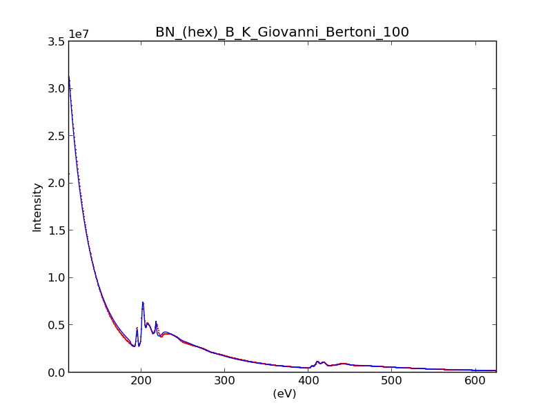
Curve fitting quantification of a boron nitride EELS core-loss spectrum from the EELS Data Base.

There are several methods that are only available in EELSModel:

• smart_fit() is a fit method that is more robust than the standard routine when fitting EELS data.

• quantify() prints the intensity at the current locations of all the EELS ionisation edges in the model.

• remove_fine_structure_data() removes the fine structure spectral data range (as defined by the fine_structure_width) ionisation edge components. It is specially useful when fitting without convolving with a zero-loss peak.

The following methods permit to easily enable/disable background and ionisation edges components:

• enable_edges()

• enable_background()

• disable_background()

• enable_fine_structure()

• disable_fine_structure()

The following methods permit to easily enable/disable several ionisation edge functionalities:

• set_all_edges_intensities_positive()

• unset_all_edges_intensities_positive()

• enable_free_onset_energy()

• disable_free_onset_energy()

• fix_edges()

• free_edges()

• fix_fine_structure()

• free_fine_structure()

When fitting edges with fine structure enabled it is often desirable that the fine structure region of nearby ionization edges does not overlap. HyperSpy provides a method, resolve_fine_structure(), to automatically adjust the fine structure to prevent fine structure to avoid overlapping. This method is executed automatically when e.g. components are added or removed from the model, but sometimes is necessary to call it manually.

Sometimes it is desirable to disable the automatic adjustment of the fine structure width. It is possible to suspend this feature by calling suspend_auto_fine_structure_width(). To resume it use suspend_auto_fine_structure_width()