Machine learning

Introduction

HyperSpy provides easy access to several “machine learning” algorithms that can be useful when analysing multi-dimensional data. In particular, decomposition algorithms, such as principal component analysis (PCA), or blind source separation (BSS) algorithms, such as independent component analysis (ICA), are available through the methods described in this section.

Hint

HyperSpy will decompose a dataset, $X$ , into two new datasets: one with the dimension of the signal space known as factors ( $A$ ), and the other with the dimension of the navigation space known as loadings ( $B$ ), such that $X = A B^T$ .

For some of the algorithms listed below, the decomposition results in an approximation of the dataset, i.e. $X \approx A B^T$ .

Decomposition

Decomposition techniques are most commonly used as a means of noise reduction (or denoising) and dimensionality reduction. To apply a decomposition to your dataset, run the decomposition() method, for example:

>>> import numpy as np
>>> from hyperspy.signals import Signal1D

>>> s = Signal1D(np.random.randn(10, 10, 200))
>>> s.decomposition()

>>> # Load data from a file, then decompose
>>> s = hs.load("my_file.hspy")
>>> s.decomposition()

Note

The signal s must be multi-dimensional, i.e. s.axes_manager.navigation_size > 1

One of the most popular uses of decomposition() is data denoising. This is achieved by using a limited set of components to make a model of the original dataset, omitting the less significant components that ideally contain only noise.

To reconstruct your denoised or reduced model, run the get_decomposition_model() method. For example:

>>> # Use all components to reconstruct the model
>>> sc = s.get_decomposition_model()

>>> # Use first 3 components to reconstruct the model
>>> sc = s.get_decomposition_model(3)

>>> # Use components [0, 2] to reconstruct the model
>>> sc = s.get_decomposition_model([0, 2])

Sometimes, it is useful to examine the residuals between your original data and the decomposition model. You can easily calculate and display the residuals, since get_decomposition_model() returns a new object, which in the example above we have called sc:

>>> (s - sc).plot()

You can perform operations on this new object sc later. It is a copy of the original s object, except that the data has been replaced by the model constructed using the chosen components.

If you provide the output_dimension argument, which takes an integer value, the decomposition algorithm attempts to find the best approximation for the dataset $X$ with only a limited set of factors $A$ and loadings $B$ , such that $X \approx A B^T$ .

>>> s.decomposition(output_dimension=3)

Some of the algorithms described below require output_dimension to be provided.

Available algorithms

HyperSpy implements a number of decomposition algorithms via the algorithm argument. The table below lists the algorithms that are currently available, and includes links to the appropriate documentation for more information on each one.

Note

Choosing which algorithm to use is likely to depend heavily on the nature of your dataset and the type of analysis you are trying to perform. We discuss some of the reasons for choosing one algorithm over another below, but would encourage you to do your own research as well. The scikit-learn documentation is a very good starting point.

Available decomposition algorithms in HyperSpy
Algorithm	Method
“SVD” (default)	`svd_pca()`
“MLPCA”	`mlpca()`
“sklearn_pca”	`sklearn.decomposition.PCA`
“NMF”	`sklearn.decomposition.NMF`
“sparse_pca”	`sklearn.decomposition.SparsePCA`
“mini_batch_sparse_pca”	`sklearn.decomposition.MiniBatchSparsePCA`
“RPCA”	`rpca_godec()`
“ORPCA”	`ORPCA`
“ORNMF”	`ORNMF`
custom object	An object implementing `fit()` and `transform()` methods

Singular value decomposition (SVD)

The default algorithm in HyperSpy is "SVD", which uses an approach called “singular value decomposition” to decompose the data in the form $X = U \Sigma V^T$ . The factors are given by $U \Sigma$ , and the loadings are given by $V^T$ . For more information, please read the method documentation for svd_pca().

>>> import numpy as np
>>> from hyperspy.signals import Signal1D

>>> s = Signal1D(np.random.randn(10, 10, 200))
>>> s.decomposition()

Note

In some fields, including electron microscopy, this approach of applying an SVD directly to the data $X$ is often called PCA (see below).

However, in the classical definition of PCA, the SVD should be applied to data that has first been “centered” by subtracting the mean, i.e. 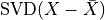$\mathrm{SVD}(X - \bar X)$ .

The "SVD" algorithm in HyperSpy does not apply this centering step by default. As a result, you may observe differences between the output of the "SVD" algorithm and, for example, sklearn.decomposition.PCA, which does apply centering.

Principal component analysis (PCA)

One of the most popular decomposition methods is principal component analysis (PCA). To perform PCA on your dataset, run the decomposition() method with any of following arguments.

If you have scikit-learn installed:

>>> s.decomposition(algorithm="sklearn_pca")

You can also turn on centering with the default "SVD" algorithm via the "centre" argument:

# Subtract the mean along the navigation axis
>>> s.decomposition(algorithm="SVD", centre="navigation")

# Subtract the mean along the signal axis
>>> s.decomposition(algorithm="SVD", centre="signal")

You can also use sklearn.decomposition.PCA directly:

>>> from sklearn.decomposition import PCA

>>> s.decomposition(algorithm=PCA())

Poissonian noise

Most of the standard decomposition algorithms assume that the noise of the data follows a Gaussian distribution (also known as “homoskedastic noise”). In cases where your data is instead corrupted by Poisson noise, HyperSpy can “normalize” the data by performing a scaling operation, which can greatly enhance the result. More details about the normalization procedure can be found in [Keenan2004].

To apply Poissonian noise normalization to your data:

>>> s.decomposition(normalize_poissonian_noise=True)

>>> # Because it is the first argument we could have simply written:
>>> s.decomposition(True)

Warning

Poisson noise normalization cannot be used in combination with data centering using the 'centre' argument. Attempting to do so will raise an error.

Maximum likelihood principal component analysis (MLPCA)

Instead of applying Poisson noise normalization to your data, you can instead use an approach known as Maximum Likelihood PCA (MLPCA), which provides a more robust statistical treatment of non-Gaussian “heteroskedastic noise”.

>>> s.decomposition(algorithm="MLPCA")

For more information, please read the method documentation for mlpca().

Note

You must set the output_dimension when using MLPCA.

Robust principal component analysis (RPCA)

PCA is known to be very sensitive to the presence of outliers in data. These outliers can be the result of missing or dead pixels, X-ray spikes, or very low count data. If one assumes a dataset, $X$ , to consist of a low-rank component $L$ corrupted by a sparse error component $S$ , such that $X=L+S$ , then Robust PCA (RPCA) can be used to recover the low-rank component for subsequent processing [Candes2011].

../_images/rpca_schematic.png — Schematic diagram of the robust PCA problem, which combines a low-rank matrix with sparse errors. Robust PCA aims to decompose the matrix back into these two components.

Note

You must set the output_dimension when using Robust PCA.

The default RPCA algorithm is GoDec [Zhou2011]. In HyperSpy it returns the factors and loadings of $L$ . RPCA solvers work by using regularization, in a similar manner to lasso or ridge regression, to enforce the low-rank constraint on the data. The low-rank regularization parameter, lambda1, defaults to 1/sqrt(n_features), but it is strongly recommended that you explore the behaviour of different values.

>>> s.decomposition(algorithm="RPCA", output_dimension=3, lambda1=0.1)

HyperSpy also implements an online algorithm for RPCA developed by Feng et al. [Feng2013]. This minimizes memory usage, making it suitable for large datasets, and can often be faster than the default algorithm.

>>> s.decomposition(algorithm="ORPCA", output_dimension=3)

The online RPCA implementation sets several default parameters that are usually suitable for most datasets, including the regularization parameter highlighted above. Again, it is strongly recommended that you explore the behaviour of these parameters. To further improve the convergence, you can “train” the algorithm with the first few samples of your dataset. For example, the following code will train ORPCA using the first 32 samples of the data.

>>> s.decomposition(algorithm="ORPCA", output_dimension=3, training_samples=32)

Finally, online RPCA includes two alternatives methods to the default block-coordinate descent solver, which can again improve both the convergence and speed of the algorithm. These are particularly useful for very large datasets.

The methods are based on stochastic gradient descent (SGD), and take an additional parameter to set the learning rate. The learning rate dictates the size of the steps taken by the gradient descent algorithm, and setting it too large can lead to oscillations that prevent the algorithm from finding the correct minima. Usually a value between 1 and 2 works well:

>>> s.decomposition(algorithm="ORPCA",
...                 output_dimension=3,
...                 method="SGD",
...                 subspace_learning_rate=1.1)

You can also use Momentum Stochastic Gradient Descent (MomentumSGD), which typically improves the convergence properties of stochastic gradient descent. This takes the further parameter “momentum”, which should be a fraction between 0 and 1.

>>> s.decomposition(algorithm="ORPCA",
...                 output_dimension=3,
...                 method="MomentumSGD",
...                 subspace_learning_rate=1.1,
...                 subspace_momentum=0.5)

Using the “SGD” or “MomentumSGD” methods enables the subspace, i.e. the underlying low-rank component, to be tracked as it changes with each sample update. The default method instead assumes a fixed, static subspace.

Non-negative matrix factorization (NMF)

Another popular decomposition method is non-negative matrix factorization (NMF), which can be accessed in HyperSpy with:

>>> s.decomposition(algorithm='NMF')

Unlike PCA, NMF forces the components to be strictly non-negative, which can aid the physical interpretation of components for count data such as images, EELS or EDS. For an example of NMF in EELS processing, see [Nicoletti2013].

NMF takes the optional argument output_dimension, which determines the number of components to keep. Setting this to a small number is recommended to keep the computation time small. Often it is useful to run a PCA decomposition first and use the scree plot to determine a suitable value for output_dimension.

Robust non-negative matrix factorization (RNMF)

In a similar manner to the online, robust methods that complement PCA above, HyperSpy includes an online robust NMF method. This is based on the OPGD (Online Proximal Gradient Descent) algorithm of [Zhao2016].

Note

You must set the output_dimension when using Robust NMF.

As before, you can control the regularization applied via the parameter “lambda1”:

>>> s.decomposition(algorithm="ORNMF", output_dimension=3, lambda1=0.1)

The MomentumSGD method is useful for scenarios where the subspace, i.e. the underlying low-rank component, is changing over time.

>>> s.decomposition(algorithm="ORNMF",
...                 output_dimension=3,
...                 method="MomentumSGD",
...                 subspace_learning_rate=1.1,
...                 subspace_momentum=0.5)

Both the default and MomentumSGD solvers assume an l2-norm minimization problem, which can still be sensitive to very heavily corrupted data. A more robust alternative is available, although it is typically much slower.

>>> s.decomposition(algorithm="ORNMF", output_dimension=3, method="RobustPGD")

Custom decomposition algorithms

HyperSpy supports passing a custom decomposition algorithm, provided it follows the form of a scikit-learn estimator. Any object that implements fit() and transform() methods is acceptable, including sklearn.pipeline.Pipeline and sklearn.model_selection.GridSearchCV. You can access the fitted estimator by passing return_info=True.

>>> # Passing a custom decomposition algorithm
>>> from sklearn.preprocessing import MinMaxScaler
>>> from sklearn.pipeline import Pipeline
>>> from sklearn.decomposition import PCA

>>> pipe = Pipeline([("scaler", MinMaxScaler()), ("PCA", PCA())])
>>> out = s.decomposition(algorithm=pipe, return_info=True)

>>> out
Pipeline(memory=None,
         steps=[('scaler', MinMaxScaler(copy=True, feature_range=(0, 1))),
                ('PCA', PCA(copy=True, iterated_power='auto', n_components=None,
                            random_state=None, svd_solver='auto', tol=0.0,
                            whiten=False))],
         verbose=False)

Blind Source Separation

In some cases it is possible to obtain more physically interpretable set of components using a process called Blind Source Separation (BSS). This largely depends on the particular application. For more information about blind source separation please see [Hyvarinen2000], and for an example application to EELS analysis, see [Pena2010].

Warning

The BSS algorithms operate on the result of a previous decomposition analysis. It is therefore necessary to perform a decomposition first before calling blind_source_separation(), otherwise it will raise an error.

You must provide an integer number_of_components argument, or a list of components as the comp_list argument. This performs BSS on the chosen number/list of components from the previous decomposition.

To perform blind source separation on the result of a previous decomposition, run the blind_source_separation() method, for example:

>>> import numpy as np
>>> from hyperspy.signals import Signal1D

>>> s = Signal1D(np.random.randn(10, 10, 200))
>>> s.decomposition(output_dimension=3)

>>> s.blind_source_separation(number_of_components=3)

# Perform only on the first and third components
>>> s.blind_source_separation(comp_list=[0, 2])

Available algorithms

HyperSpy implements a number of BSS algorithms via the algorithm argument. The table below lists the algorithms that are currently available, and includes links to the appropriate documentation for more information on each one.

Available blind source separation algorithms in HyperSpy
Algorithm	Method
“sklearn_fastica” (default)	`sklearn.decomposition.FastICA`
“orthomax”	`orthomax()`
“FastICA”	`mdp.nodes.FastICANode`
“JADE”	`mdp.nodes.JADENode`
“CuBICA”	`mdp.nodes.CuBICANode`
“TDSEP”	`mdp.nodes.TDSEPNode`
custom object	An object implementing `fit()` and `transform()` methods

Note

Except orthomax(), all of the implemented BSS algorithms listed above rely on external packages being available on your system. sklearn_fastica, requires scikit-learn while FastICA, JADE, CuBICA, TDSEP require the Modular toolkit for Data Processing (MDP).

Orthomax

Orthomax rotations are a statistical technique used to clarify and highlight the relationship among factors, by adjusting the coordinates of PCA results. The most common approach is known as “varimax”, which intended to maximize the variance shared among the components while preserving orthogonality. The results of an orthomax rotation following PCA are often “simpler” to interpret than just PCA, since each componenthas a more discrete contribution to the data.

>>> import numpy as np
>>> from hyperspy.signals import Signal1D

>>> s = Signal1D(np.random.randn(10, 10, 200))
>>> s.decomposition(output_dimension=3)

>>> s.blind_source_separation(number_of_components=3, algorithm="orthomax")

Independent component analysis (ICA)

One of the most common approaches for blind source separation is Independent Component Analysis (ICA). This separates a signal into subcomponents by assuming that the subcomponents are (a) non-Gaussian, and (b) that they are statistically independent from each other.

Custom BSS algorithms

As with decomposition, HyperSpy supports passing a custom BSS algorithm, provided it follows the form of a scikit-learn estimator. Any object that implements fit() and transform() methods is acceptable, including sklearn.pipeline.Pipeline and sklearn.model_selection.GridSearchCV. You can access the fitted estimator by passing return_info=True.

>>> # Passing a custom BSS algorithm
>>> from sklearn.preprocessing import MinMaxScaler
>>> from sklearn.pipeline import Pipeline
>>> from sklearn.decomposition import FastICA

>>> pipe = Pipeline([("scaler", MinMaxScaler()), ("ica", FastICA())])
>>> out = s.blind_source_separation(number_of_components=3, algorithm=pipe, return_info=True)

>>> out
Pipeline(memory=None,
         steps=[('scaler', MinMaxScaler(copy=True, feature_range=(0, 1))),
                ('ica', FastICA(algorithm='parallel', fun='logcosh', fun_args=None,
                                max_iter=200, n_components=3, random_state=None,
                                tol=0.0001, w_init=None, whiten=True))],
         verbose=False)

Cluster analysis

New in version 1.6.

Introduction

Cluster analysis or clustering is the task of grouping a set of measurements such that measurements in the same group (called a cluster) are more similar (in some sense) to each other than to those in other groups (clusters). A HyperSpy signal can represent a number of large arrays of different measurements which can represent spectra, images or sets of paramaters. Identifying and extracting trends from large datasets is often difficult and decomposition methods, blind source separation and cluster analysis play an important role in this process.

Cluster analysis, in essence, compares the “distances” (or similar metric) between different sets of measurements and groups those that are closest together. The features it groups can be raw data points, for example, comparing for every navigation dimension all points of a spectrum. However, if the dataset is large, the process of clustering can be computationally intensive so clustering is more commonly used on an extracted set of features or parameters. For example, extraction of two peak positions of interest via a fitting process rather than clustering all spectra points.

In favourable cases, matrix decomposition and related methods can decompose the data into a (ideally small) set of significant loadings and factors. The factors capture a core representation of the features in the data and the loadings provide the mixing ratios of these factors that best describe the original data. Overall, this usually represents a much smaller data volume compared to the original data and can helps to identify correlations.

A detailed description of the application of cluster analysis in x-ray spectro-microscopy and further details on the theory and implementation can be found in [Lerotic2004].

Nomenclature

Taking the example of a 1D Signal of dimensions (20, 10|4) containing the dataset, we say there are 200 samples. The four measured parameters are the features. If we choose to search for 3 clusters within this dataset, we derive three main values:

The labels, of dimensions (3| 20, 10). Each navigation position is assigned to a cluster. The labels of each cluster are boolean arrays that mark the data that has been assigned to the cluster with True.
The cluster_distances, of dimensions (3| 20, 10), which are the distances of all the data points to the centroid of each cluster.
The “cluster signals”, which are signals that are representative of their clusters. In HyperSpy two are computer: cluster_sum_signals and cluster_centroid_signals, of dimensions (3| 4), which are the sum of all the cluster signals that belong to each cluster or the signal closest to each cluster centroid respectively.

Clustering functions HyperSpy

All HyperSpy signals have the following methods for clustering analysis:

cluster_analysis()
plot_cluster_results()
plot_cluster_labels()
plot_cluster_signals()
plot_cluster_distances()
get_cluster_signals()
get_cluster_labels()
get_cluster_distances()
estimate_number_of_clusters()
plot_cluster_metric()

The cluster_analysis() method can perform cluster analysis using any sklearn.clustering clustering algorithms or any other object with a compatible API. This involves importing the relevant algorithm class from scikit-learn.

>>> from sklearn.cluster import KMeans
>>> s.cluster_analysis(cluster_source="signal", algorithm=KMeans(n_clusters=3, n_init=8))

For convenience, the default algorithm is kmeans algorithm and is imported internally. All extra keyword arguments are passed to the algorithm when present. Therefore the following code is equivalent to the previous one:

For example:

>>> s.cluster_analysis(cluster_source="signal", n_clusters=3, preprocessing="norm", algorithm="kmeans", n_init=8)

is equivalent to:

cluster_analysis() computes the cluster labels. The clusters areas with identical label are averaged to create a set of cluster centres. This averaging can be performed on the signal itself, the bss or decomposition results or a user supplied signal.

Pre-processing

Cluster analysis measures the distances between features and groups them. It is often necessary to pre-process the features in order to obtain meaningful results.

For example, pre-processing can be useful to reveal clusters when performing cluster analysis of decomposition results. Decomposition methods decompose data into a set of factors and a set of loadings defining the mixing needed to represent the data. If signal 1 is reduced to three components with mixing 0.1 0.5 2.0, and signal 2 is reduced to a mixing of 0.2 1.0 4.0, it should be clear that these represent the same signal but with a scaling difference. Normalization of the data can again be used to remove scaling effects.

Therefore, the pre-processing step will highly influence the results and should be evaluated for the problem under investigation.

All pre-processing methods from (or compatible with) sklearn.preprocessing can be passed to the scaling keyword of the cluster_analysis() method. For convenience, the following methods from scikit-learn are available as standard: standard , minmax and norm as standard. Briefly, norm treats the features as a vector and normalizes the vector length. standard re-scales each feature by removing the mean and scaling to unit variance. minmax normalizes each feature between the minimum and maximum range of that feature.

Cluster signals

In HyperSpy cluster signals are signals that somehow represent their clusters. The concept is ill-defined, since cluster algorithms only assign data points to clusters. HyperSpy computers 2 cluster signals,

cluster_sum_signals, which are the sum of all the cluster signals that belong to each cluster.
cluster_centroid_signals, which is the signal closest to each cluster centroid.

When plotting the “cluster signals” we can select any of those above using the signal keyword argument:

>>> s.plot_cluster_labels(signal="centroid")

In addition, it is possible to plot the mean signal over the different clusters:

>>> s.plot_cluster_labels(signal="mean")

Clustering with user defined algorithms

User developed preprocessing or cluster algorithms can be used in place of the sklearn methods. A preprocessing object needs a fit_transform which appropriately scales the data. The example below defines a preprocessing class which normalizes the data then applies a square root to enhances weaker features.

>>> class PowerScaling(object):
>>>
>>>     def __init__(self,power=0.5):
>>>         self.power = power
>>>
>>>     def fit_transform(self,data):
>>>         norm = np.amax(data,axis=1)
>>>         scaled_data = data/norm[:,None]
>>>         scaled_data = scaled_data - np.min(scaled_data)+1.0e-8
>>>         scaled_data = scaled_data ** self.power
>>>         return scaled_data

The PowerScaling class can then be passed to the cluster_analysis method for use.

>>> ps = PowerScaling()
>>> s.cluster_analysis(cluster_source="decomposition", number_of_components=3, preprocessing=ps)

For user defined clustering algorithms the class must implementation fit and have a label_ attribute that contains the clustering labels. An example template would be:

>>> class MyClustering(object):
>>>
>>>     def __init__(self):
>>>         self.labels_ = None
>>>
>>>     def fit_(self,X):
>>>         self.labels_ = do_something(X)

Examples

Clustering using decomposition results

Let’s use the make_blobs function supplied by scikit-learn to make dummy data to see how clustering might work in practice.

>>> import hyperspy.api as hs
>>> from sklearn.datasets import make_blobs
>>> data = make_blobs(
>>>         n_samples=1000,
>>>         n_features=100,
>>>         centers=3,
>>>         shuffle=False,
>>>         random_state=1)[0].reshape(50, 20, 100)
>>> s = hs.signals.Signal1D(data)

>>> hs.plot.plot_images(data.T)

To see how cluster analysis works it’s best to first examine the signal. Moving around the image you should be able to see 3 distinct regions in which the 1D signal modulates slightly.

>>> s.plot()

Let’s perform SVD to reduce the dimensionality of the dataset by exploiting redundancies:

>>> s.decomposition()
>>> s.plot_explained_variance_ratio()

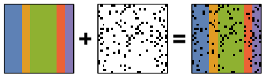
From the scree plot we deduce that, as expected, that the dataset can be reduce to 3 components. Let’s plot their loadings:

>>> s.plot_decomposition_loadings(comp_ids=3, axes_decor="off")

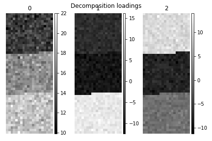
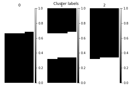
../_images/clustering_decomposition_loadings.png

In the SVD loading we can identify 3 regions, but they are mixed in the components. Let’s perform cluster analysis of decomposition results, to find similar regions and the representative features in those regions. Notice that this dataset does not require any pre-processing for cluster analysis.

>>> s.cluster_analysis(cluster_source="decomposition", number_of_components=3, preprocessing=None)
>>> s.plot_cluster_labels(axes_decor="off")

To see what the labels the cluster algorithm has assigned you can inspect the cluster_labels:

>>> s.learning_results.cluster_labels[0]
array([0, 0, 0, 0, 0, 0, 0, 0, 0, 0, 0, 0, 0, 0, 0, 0, 0, 0, 0, 0, 0, 0,
   0, 0, 0, 0, 0, 0, 0, 0, 0, 0, 0, 0, 0, 0, 0, 0, 0, 0, 0, 0, 0, 0,
   0, 0, 0, 0, 0, 0, 0, 0, 0, 0, 0, 0, 0, 0, 0, 0, 0, 0, 0, 0, 0, 0,
   0, 0, 0, 0, 0, 0, 0, 0, 0, 0, 0, 0, 0, 0, 0, 0, 0, 0, 0, 0, 0, 0,
   0, 0, 0, 0, 0, 0, 0, 0, 0, 0, 0, 0, 0, 0, 0, 0, 0, 0, 0, 0, 0, 0,
   0, 0, 0, 0, 0, 0, 0, 0, 0, 0, 0, 0, 0, 0, 0, 0, 0, 0, 0, 0, 0, 0,
   0, 0, 0, 0, 0, 0, 0, 0, 0, 0, 0, 0, 0, 0, 0, 0, 0, 0, 0, 0, 0, 0,
   0, 0, 0, 0, 0, 0, 0, 0, 0, 0, 0, 0, 0, 0, 0, 0, 0, 0, 0, 0, 0, 0,
   0, 0, 0, 0, 0, 0, 0, 0, 0, 0, 0, 0, 0, 0, 0, 0, 0, 0, 0, 0, 0, 0,
   0, 0, 0, 0, 0, 0, 0, 0, 0, 0, 0, 0, 0, 0, 0, 0, 0, 0, 0, 0, 0, 0,
   0, 0, 0, 0, 0, 0, 0, 0, 0, 0, 0, 0, 0, 0, 0, 0, 0, 0, 0, 0, 0, 0,
   0, 0, 0, 0, 0, 0, 0, 0, 0, 0, 0, 0, 0, 0, 0, 0, 0, 0, 0, 0, 0, 0,
   0, 0, 0, 0, 0, 0, 0, 0, 0, 0, 0, 0, 0, 0, 0, 0, 0, 0, 0, 0, 0, 0,
   0, 0, 0, 0, 0, 0, 0, 0, 0, 0, 0, 0, 0, 0, 0, 0, 0, 0, 0, 0, 0, 0,
   0, 0, 0, 0, 0, 0, 0, 0, 0, 0, 0, 0, 0, 0, 0, 0, 0, 0, 0, 0, 0, 0,
   0, 0, 0, 0, 1, 1, 1, 1, 1, 1, 1, 1, 1, 1, 1, 1, 1, 1, 1, 1, 1, 1,
   1, 1, 1, 1, 1, 1, 1, 1, 1, 1, 1, 1, 1, 1, 1, 1, 1, 1, 1, 1, 1, 1,
   1, 1, 1, 1, 1, 1, 1, 1, 1, 1, 1, 1, 1, 1, 1, 1, 1, 1, 1, 1, 1, 1,
   1, 1, 1, 1, 1, 1, 1, 1, 1, 1, 1, 1, 1, 1, 1, 1, 1, 1, 1, 1, 1, 1,
   1, 1, 1, 1, 1, 1, 1, 1, 1, 1, 1, 1, 1, 1, 1, 1, 1, 1, 1, 1, 1, 1,
   1, 1, 1, 1, 1, 1, 1, 1, 1, 1, 1, 1, 1, 1, 1, 1, 1, 1, 1, 1, 1, 1,
   1, 1, 1, 1, 1, 1, 1, 1, 1, 1, 1, 1, 1, 1, 1, 1, 1, 1, 1, 1, 1, 1,
   1, 1, 1, 1, 1, 1, 1, 1, 1, 1, 1, 1, 1, 1, 1, 1, 1, 1, 1, 1, 1, 1,
   1, 1, 1, 1, 1, 1, 1, 1, 1, 1, 1, 1, 1, 1, 1, 1, 1, 1, 1, 1, 1, 1,
   1, 1, 1, 1, 1, 1, 1, 1, 1, 1, 1, 1, 1, 1, 1, 1, 1, 1, 1, 1, 1, 1,
   1, 1, 1, 1, 1, 1, 1, 1, 1, 1, 1, 1, 1, 1, 1, 1, 1, 1, 1, 1, 1, 1,
   1, 1, 1, 1, 1, 1, 1, 1, 1, 1, 1, 1, 1, 1, 1, 1, 1, 1, 1, 1, 1, 1,
   1, 1, 1, 1, 1, 1, 1, 1, 1, 1, 1, 1, 1, 1, 1, 1, 1, 1, 1, 1, 1, 1,
   1, 1, 1, 1, 1, 1, 1, 1, 1, 1, 1, 1, 1, 1, 1, 1, 1, 1, 1, 1, 1, 1,
   1, 1, 1, 1, 1, 1, 1, 1, 1, 1, 1, 1, 1, 1, 1, 1, 1, 1, 1, 1, 1, 1,
   1, 1, 1, 1, 1, 1, 1, 0, 0, 0, 0, 0, 0, 0, 0, 0, 0, 0, 0, 0, 0, 0,
   0, 0, 0, 0, 0, 0, 0, 0, 0, 0, 0, 0, 0, 0, 0, 0, 0, 0, 0, 0, 0, 0,
   0, 0, 0, 0, 0, 0, 0, 0, 0, 0, 0, 0, 0, 0, 0, 0, 0, 0, 0, 0, 0, 0,
   0, 0, 0, 0, 0, 0, 0, 0, 0, 0, 0, 0, 0, 0, 0, 0, 0, 0, 0, 0, 0, 0,
   0, 0, 0, 0, 0, 0, 0, 0, 0, 0, 0, 0, 0, 0, 0, 0, 0, 0, 0, 0, 0, 0,
   0, 0, 0, 0, 0, 0, 0, 0, 0, 0, 0, 0, 0, 0, 0, 0, 0, 0, 0, 0, 0, 0,
   0, 0, 0, 0, 0, 0, 0, 0, 0, 0, 0, 0, 0, 0, 0, 0, 0, 0, 0, 0, 0, 0,
   0, 0, 0, 0, 0, 0, 0, 0, 0, 0, 0, 0, 0, 0, 0, 0, 0, 0, 0, 0, 0, 0,
   0, 0, 0, 0, 0, 0, 0, 0, 0, 0, 0, 0, 0, 0, 0, 0, 0, 0, 0, 0, 0, 0,
   0, 0, 0, 0, 0, 1, 0, 0, 0, 0, 0, 0, 0, 0, 0, 0, 0, 0, 0, 0, 0, 0,
   0, 0, 0, 0, 0, 0, 0, 0, 0, 0, 0, 0, 0, 0, 0, 0, 0, 0, 0, 0, 0, 0,
   0, 0, 0, 0, 0, 0, 0, 0, 0, 0, 0, 0, 0, 0, 0, 0, 0, 0, 0, 0, 0, 0,
   0, 0, 0, 0, 0, 0, 0, 0, 0, 0, 0, 0, 0, 0, 0, 0, 0, 0, 0, 0, 0, 0,
   0, 0, 0, 0, 0, 0, 0, 0, 0, 0, 0, 0, 0, 0, 0, 0, 0, 0, 0, 0, 0, 0,
   0, 0, 0, 0, 0, 0, 0, 0, 0, 0, 0, 0, 0, 0, 0, 0, 0, 0, 0, 0, 0, 0,
   0, 0, 0, 0, 0, 0, 0, 0, 0, 0])

In this case we know there are 3 cluster, but for real examples the number of clusters is not known a priori. A number of metrics, such as elbow, Silhouette and Gap can be used to estimate the optimal number of clusters. The elbow method measures the sum-of-squares of the distances within a cluster and, as for the PCA decomposition, an “elbow” or point where the gains diminish with increasing number of clusters indicates the ideal number of clusters. Silhouette analysis measures how well separated clusters are and can be used to determine the most likely number of clusters. As the scoring is a measure of separation of clusters a number of solutions may occur and maxima in the scores are used to indicate possible solutions. Gap analysis is similar but compares the “gap” between the clustered data results and those from a randomly data set of the same size. The largest gap indicates the best clustering. The metric results can be plotted to check how well-defined the clustering is.

>>> s.estimate_number_of_clusters(cluster_source="decomposition", metric="gap")
>>> s.plot_cluster_metric()

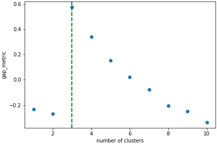
The optimal number of clusters can be set or accessed from the learning results

>>> s.learning_results.number_of_clusters
3

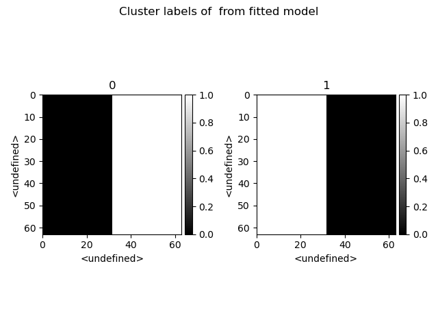
Clustering using another signal as source

In this example we will perform clustering analysis on the position of two peaks. The signals containing the position of the peaks can be computed for example using curve fitting. Given an existing fitted model, the parameters can be extracted as signals and stacked. Clustering can then be applied as described previously to identify trends in the fitted results.

Let’s start by creating a suitable synthetic dataset.

>>> import hyperspy.api as hs
>>> import numpy as np
>>> s_dummy = hs.signals.Signal1D(np.zeros((64, 64, 1000)))
>>> s_dummy.axes_manager.signal_axes[0].scale = 2e-3
>>> s_dummy.axes_manager.signal_axes[0].units = "eV"
>>> s_dummy.axes_manager.signal_axes[0].name = "energy"
>>> m = s_dummy.create_model()
>>> m.append(hs.model.components1D.GaussianHF(fwhm=0.2))
>>> m.append(hs.model.components1D.GaussianHF(fwhm=0.3))
>>> m.components.GaussianHF.centre.map["values"][:32, :] = .3 + .1
>>> m.components.GaussianHF.centre.map["values"][32:, :] = .7 + .1
>>> m.components.GaussianHF_0.centre.map["values"][:, 32:] = m.components.GaussianHF.centre.map["values"][:, 32:] * 2
>>> m.components.GaussianHF_0.centre.map["values"][:, :32] = m.components.GaussianHF.centre.map["values"][:, :32] * 0.5
>>> for component in m:
...     component.centre.map["is_set"][:] = True
...     component.centre.map["values"][:] += np.random.normal(size=(64, 64)) * 0.01
>>> s = m.as_signal()
>>> stack = hs.stack([m.components.GaussianHF.centre.as_signal(),
>>> hs.plot.plot_images(stack, axes_decor="off", colorbar="single",
suptitle="")

../_images/clustering_gaussian_centres.png

Let’s now perform cluster analysis on the stack and calculate the centres using the spectrum image. Notice that we don’t need to fit the model to the data because this is a synthetic dataset. When analysing experimental data you will need to fit the model first. Also notice that here we need to pre-process the dataset by normalization in order to reveal the clusters due to the proportionality relationship between the position of the peaks.

>>> stack = hs.stack([m.components.GaussianHF.centre.as_signal(),
m.components.GaussianHF_0.centre.as_signal()])
>>> s.estimate_number_of_clusters(cluster_source=stack.T, preprocessing="norm")
2
>>> s.cluster_analysis(cluster_source=stack.T, source_for_centers=s, n_clusters=2, preprocessing="norm")
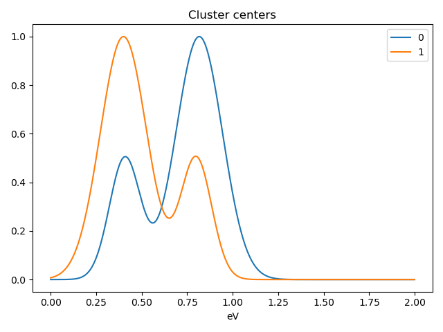
>>> s.plot_cluster_labels()

../_images/clustering_gaussian_centres_labels.png

>>> s.plot_cluster_signals(signal="mean")

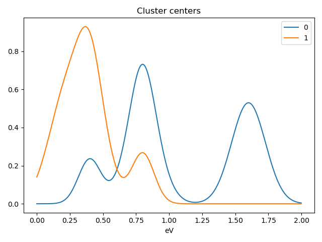
../_images/clustering_gaussian_centres_mean.png

Notice that in this case averaging or summing the signals of each cluster is not appropriate, since the clustering criterium is the ratio between the peaks positions. A better alternative is to plot the signals closest to the centroids:

>>> s.plot_cluster_signals(signal="centroid")

../_images/clustering_gaussian_centres_centroid.png

Visualizing results

HyperSpy includes a number of plotting methods for visualizing the results of decomposition and blind source separation analyses. All the methods begin with plot_.

Scree plots

Note

Scree plots are only available for the "SVD" and "PCA" algorithms.

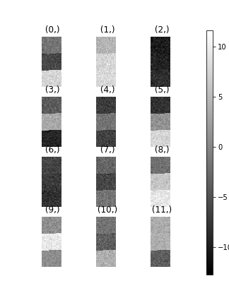
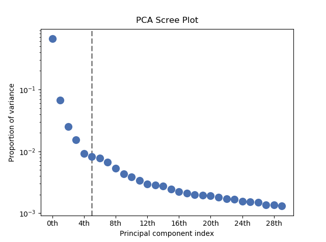
PCA will sort the components in the dataset in order of decreasing variance. It is often useful to estimate the dimensionality of the data by plotting the explained variance against the component index. This plot is sometimes called a scree plot. For most datasets, the values in a scree plot will decay rapidly, eventually becoming a slowly descending line.

To obtain a scree plot for your dataset, run the plot_explained_variance_ratio() method:

>>> s.plot_explained_variance_ratio(n=20)

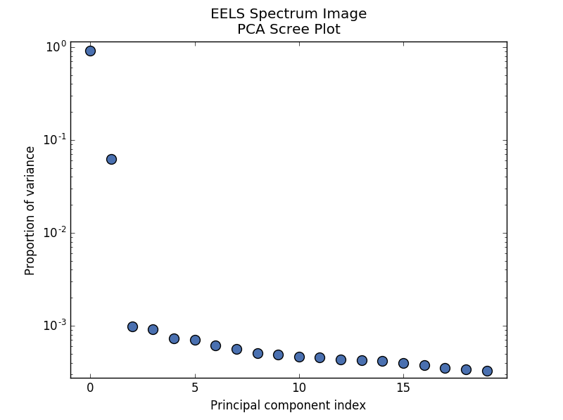
../_images/screeplot.png — PCA scree plot

The point at which the scree plot becomes linear (often referred to as the “elbow”) is generally judged to be a good estimation of the dimensionality of the data (or equivalently, the number of components that should be retained - see below). Components to the left of the elbow are considered part of the “signal”, while components to the right are considered to be “noise”, and thus do not explain any significant features of the data.

By specifying a threshold value, a cutoff line will be drawn at the total variance specified, and the components above this value will be styled distinctly from the remaining components to show which are considered signal, as opposed to noise. Alternatively, by providing an integer value for threshold, the line will be drawn at the specified component (see below).

Note that in the above scree plot, the first component has index 0. This is because Python uses zero-based indexing. To switch to a “number-based” (rather than “index-based”) notation, specify the xaxis_type parameter:

>>> s.plot_explained_variance_ratio(n=20, threshold=4, xaxis_type='number')

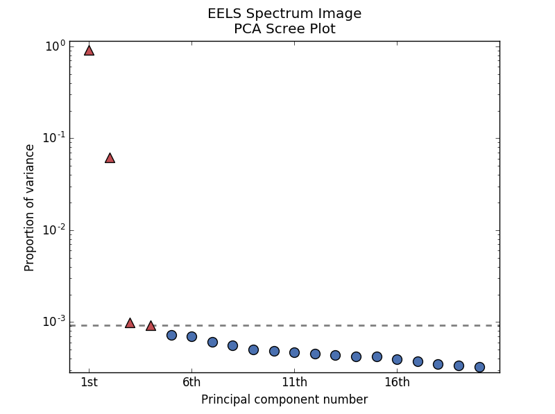
../_images/screeplot2.png — PCA scree plot with number-based axis labeling and a threshold value specified

The number of significant components can be estimated and a vertical line drawn to represent this by specifying vline=True. In this case, the “elbow” is found in the variance plot by estimating the distance from each point in the variance plot to a line joining the first and last points of the plot, and then selecting the point where this distance is largest.

If multiple maxima are found, the index corresponding to the first occurrence is returned. As the index of the first component is zero, the number of significant PCA components is the elbow index position + 1. More details about the elbow-finding technique can be found in [Satopää2011], and in the documentation for estimate_elbow_position().

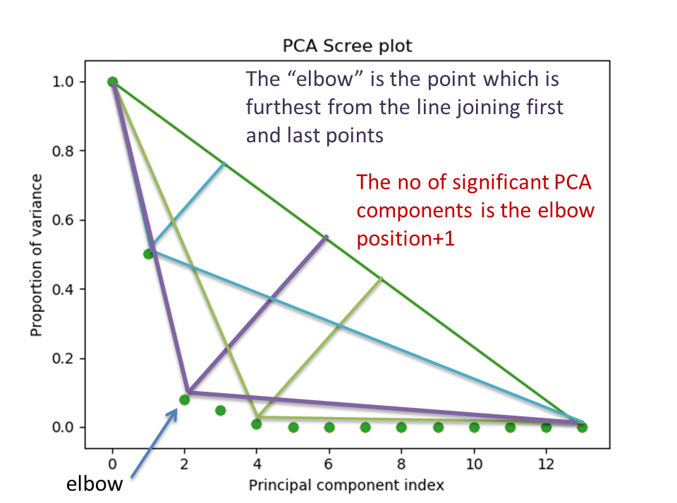
../_images/screeplot3.png — PCA scree plot with number-based axis labeling and an estimate of the no of significant positions based on the “elbow” position

These options (together with many others), can be customized to develop a figure of your liking. See the documentation of plot_explained_variance_ratio() for more details.

Sometimes it can be useful to get the explained variance ratio as a spectrum. For example, to plot several scree plots obtained with different data pre-treatments in the same figure, you can combine plot_spectra() with get_explained_variance_ratio().

Decomposition plots

HyperSpy provides a number of methods for visualizing the factors and loadings found by a decomposition analysis. To plot everything in a compact form, use plot_decomposition_results().

You can also plot the factors and loadings separately using the following methods. It is recommended that you provide the number of factors or loadings you wish to visualise, since the default is to plot all of them.

plot_decomposition_factors()
plot_decomposition_loadings()

Clustering plots

Visualizing cluster results is much the same as decomposition. You can use plot_bss_results() for a compact display, or instead:

plot_cluster_results().
plot_cluster_signals().
plot_cluster_labels().

Obtaining the results as BaseSignal instances

The decomposition and BSS results are internally stored as numpy arrays in the BaseSignal class. Frequently it is useful to obtain the decomposition/BSS factors and loadings as HyperSpy signals, and HyperSpy provides the following methods for that purpose:

get_decomposition_loadings()
get_decomposition_factors()
get_bss_loadings()
get_bss_factors()

Saving and loading results

Saving in the main file

If you save the dataset on which you’ve performed machine learning analysis in the HSpy - HyperSpy’s HDF5 Specification format (the default in HyperSpy) (see Saving data to files), the result of the analysis is also saved in the same file automatically, and it is loaded along with the rest of the data when you next open the file.

Note

This approach currently supports storing one decomposition and one BSS result, which may not be enough for your purposes.

Saving to an external file

Alternatively, you can save the results of the current machine learning analysis to a separate file with the save() method:

>>> # Save the result of the analysis
>>> s.learning_results.save('my_results.npz')

>>> # Load back the results
>>> s.learning_results.load('my_results.npz')

Exporting in different formats

You can also export the results of a machine learning analysis to any format supported by HyperSpy with the following methods:

export_decomposition_results()
export_bss_results()

These methods accept many arguments to customise the way in which the data is exported, so please consult the method documentation. The options include the choice of file format, the prefixes for loadings and factors, saving figures instead of data and more.

Warning

Data exported in this way cannot be easily loaded into HyperSpy’s machine learning structure.

Machine learning

Introduction

Decomposition

Available algorithms

Singular value decomposition (SVD)

Principal component analysis (PCA)

Poissonian noise

Maximum likelihood principal component analysis (MLPCA)

Robust principal component analysis (RPCA)

Non-negative matrix factorization (NMF)

Robust non-negative matrix factorization (RNMF)

Custom decomposition algorithms

Blind Source Separation

Available algorithms

Orthomax

Independent component analysis (ICA)

Custom BSS algorithms

Cluster analysis

Introduction

Nomenclature

Clustering functions HyperSpy

Pre-processing

Cluster signals

Clustering with user defined algorithms

Examples

Clustering using decomposition results

Clustering using another signal as source

Visualizing results

Scree plots

Decomposition plots

Blind source separation plots

Clustering plots

Obtaining the results as BaseSignal instances

Saving and loading results

Saving in the main file

Saving to an external file

Exporting in different formats