Component convolution

This example illustrates the convolution steps in the implementation of convolution in model fitting.

import hyperspy.api as hs
import numpy as np

from hyperspy.misc.axis_tools import calculate_convolution1D_axis

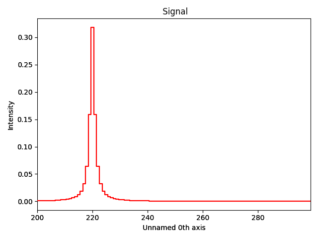
Create a signal containing a Lorentzian peak:

f = hs.model.components1D.Lorentzian(centre=220)
f_signal = hs.signals.Signal1D(f.function(np.arange(200, 300)))
f_signal.axes_manager.signal_axes.set(offset=200)
f_signal.plot()

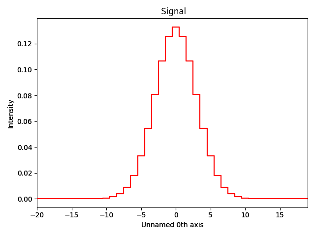
Create a second signal, for example a detector response:

g = hs.model.components1D.Gaussian(sigma=3)
g_signal = hs.signals.Signal1D(g.function(np.arange(-20, 20)))
g_signal.axes_manager.signal_axes.set(offset=-20)
g_signal.plot()

Create the “convolution axis” which adds the necessary padding:

convolution_axis = calculate_convolution1D_axis(
    f_signal.axes_manager.signal_axes[0], g_signal.axes_manager.signal_axes[0]
    )

Extend the data over the full range of the “convolution axis” and take the convolution with g_signal:

f_padded_data = f.function(convolution_axis)
convolved_data = np.convolve(f_padded_data, g_signal.data, mode="valid")

convolved_signal = hs.signals.Signal1D(convolved_data)
convolved_signal.axes_manager.signal_axes.set(offset=f_signal.axes_manager[-1].offset)

Display the comparison of both signals:

hs.plot.plot_spectra([f_signal, convolved_signal])

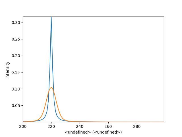
<Axes: xlabel='<undefined> (<undefined>)', ylabel='Intensity'>