Plotting spectra with different y-axis scales

The plot_spectra() function supports the yscale argument to plot spectra with any of the y-axis scales provided by matplotlib.scale: in addition to the commonly used 'linear' and 'log' scales, the 'symlog', 'asinh', 'logit', 'function' and 'functionlog' scales are also available with the 'overlap', 'cascade' and 'mosaic' styles.

The parameters specific to each scale (for example linthresh for the 'symlog' scale) are passed as keyword arguments, following the matplotlib.axes.Axes.set_yscale() API. With the 'heatmap' style, the yscale argument is passed as the norm argument of plot().

First, we simulate a few spectra with values spanning several orders of magnitude, as typically obtained with, for example, EELS or CL data.

import numpy as np

import hyperspy.api as hs

rng = np.random.default_rng(1)
wavelength = np.linspace(400, 900, 350)
spectra = []
for amplitude, decay in [(120, 80), (80, 150), (40, 250)]:
    data = amplitude * np.exp(-(wavelength - 400) / decay) + rng.poisson(
        0.2, wavelength.size
    )
    spectra.append(hs.signals.Signal1D(data))
    spectra[-1].axes_manager[0].name = "Wavelength"
    spectra[-1].axes_manager[0].units = "nm"

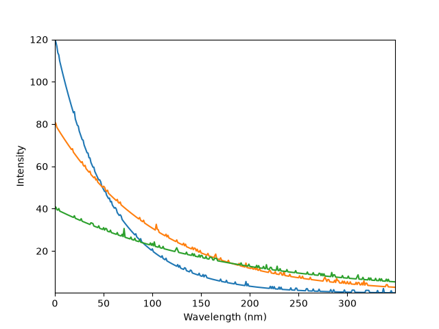
By default, the y-axis uses a 'linear' scale, which hides the detail of the low-intensity features.

hs.plot.plot_spectra(spectra, style="overlap")

<Axes: xlabel='Wavelength (nm)', ylabel='Intensity'>

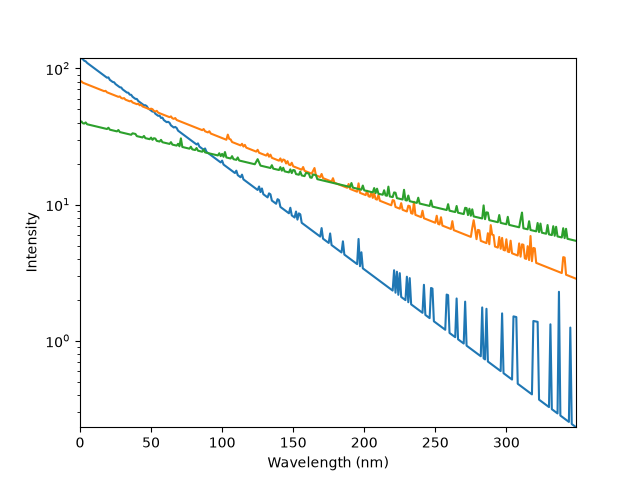
The same data plotted with a logarithmic y-axis scale makes the low-intensity part of the spectra readable.

hs.plot.plot_spectra(spectra, style="overlap", yscale="log")

<Axes: xlabel='Wavelength (nm)', ylabel='Intensity'>

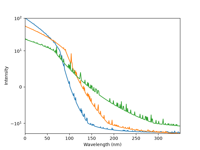
The 'symlog' scale is useful when the data spans several orders of magnitude around zero: the linthresh argument defines the range (-linthresh to linthresh) within which the scale is linear.

spectra_shifted = [s - s.data.mean() for s in spectra]

hs.plot.plot_spectra(spectra_shifted, style="overlap", yscale="symlog", linthresh=10)

<Axes: xlabel='Wavelength (nm)', ylabel='Intensity'>

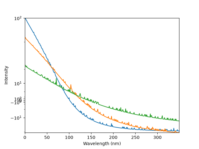
Alternatively, the 'asinh' scale is similar to the 'symlog' scale, but with a smoother transition between the linear and logarithmic regions, the width of which is set with the linear_width argument.

hs.plot.plot_spectra(spectra_shifted, style="overlap", yscale="asinh", linear_width=20)

<Axes: xlabel='Wavelength (nm)', ylabel='Intensity'>

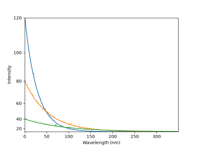
Custom scales can also be used with the 'function' and 'functionlog' scales by passing the functions argument: in this case, the y-axis follows the square of the values.

def forward(x):
    return x**2


def inverse(x):
    return x ** (1 / 2)


hs.plot.plot_spectra(
    spectra, style="overlap", yscale="function", functions=(forward, inverse)
)

<Axes: xlabel='Wavelength (nm)', ylabel='Intensity'>

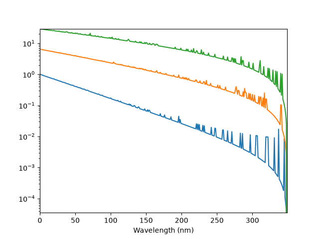
The 'cascade' style supports the 'linear', 'log' and 'symlog' scales.

hs.plot.plot_spectra(spectra, style="cascade", yscale="log")

<Axes: xlabel='Wavelength (nm)'>

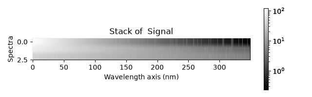
Finally, when plotting with the 'heatmap' style, the yscale argument is passed as the norm argument of plot().

hs.plot.plot_spectra(spectra, style="heatmap", yscale="log")

• 
• 

  0%|          | 0/7 [00:00<?, ?it/s]
100%|██████████| 7/7 [00:00<00:00, 5319.83it/s]

<Axes: title={'center': 'Stack of  Signal'}, xlabel='Wavelength axis (nm)', ylabel='Spectra'>