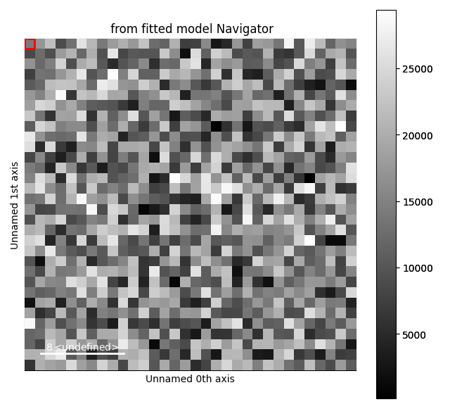
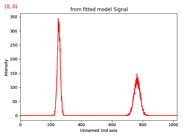
Simple simulation (2 Gaussians)

Creates a 2D hyperspectrum consisting of two Gaussians and plots it.

This example can serve as starting point to test other functionalities on the simulated hyperspectrum.

• 
• 

import numpy as np
import hyperspy.api as hs
import matplotlib.pyplot as plt


# Create an empty spectrum
s = hs.signals.Signal1D(np.zeros((32, 32, 1024)))

# Generate some simple data: two Gaussians with random centers and area

# First we create a model
m = s.create_model()

# Define the first gaussian
gs1 = hs.model.components1D.Gaussian()
# Add it to the model
m.append(gs1)

# Set the parameters
m.set_parameters_value('sigma', 10, component_list=[gs1])
# Make the center vary in the -5,5 range around 128
gs1.centre.map['values'][:] = 256 + (np.random.random((32, 32)) - 0.5) * 10
gs1.centre.map['is_set'][:] = True

# Make the area vary between 0 and 10000
gs1.A.map['values'][:] = 10000 * np.random.random((32, 32))
gs1.A.map['is_set'][:] = True

# Second gaussian
gs2 = hs.model.components1D.Gaussian()
# Add it to the model
m.append(gs2)

# Set the parameters
m.set_parameters_value('sigma', 20, component_list=[gs2])

# Make the center vary in the -10,10 range around 768
gs2.centre.map['values'][:] = 768 + (np.random.random((32, 32)) - 0.5) * 20
gs2.centre.map['is_set'][:] = True

# Make the area vary between 0 and 20000
gs2.A.map['values'][:] = 20000 * np.random.random((32, 32))
gs2.A.map['is_set'][:] = True

# Create the dataset
s_model = m.as_signal()

# Add noise
s_model.set_signal_origin("simulation")
s_model.add_poissonian_noise()

# Plot the result
s_model.plot()

plt.show()